This page was generated from ad/methods/adversarialae.ipynb.
Adversarial Auto-Encoder
Overview
The adversarial detector follows the method explained in the Adversarial Detection and Correction by Matching Prediction Distributions paper. Usually, autoencoders are trained to find a transformation \(T\) that reconstructs the input instance \(x\) as accurately as possible with loss functions that are suited to capture the similarities between x and \(x'\) such as the mean squared reconstruction error. The novelty of the adversarial autoencoder (AE) detector relies on the use of a classification model-dependent loss function based on a distance metric in the output space of the model to train the autoencoder network. Given a classification model \(M\) we optimise the weights of the autoencoder such that the KL-divergence between the model predictions on \(x\) and on \(x'\) is minimised. Without the presence of a reconstruction loss term \(x'\) simply tries to make sure that the prediction probabilities \(M(x')\) and \(M(x)\) match without caring about the proximity of \(x'\) to \(x\). As a result, \(x'\) is allowed to live in different areas of the input feature space than \(x\) with different decision boundary shapes with respect to the model \(M\). The carefully crafted adversarial perturbation which is effective around x does not transfer to the new location of \(x'\) in the feature space, and the attack is therefore neutralised. Training of the autoencoder is unsupervised since we only need access to the model prediction probabilities and the normal training instances. We do not require any knowledge about the underlying adversarial attack and the classifier weights are frozen during training.
The detector can be used as follows:
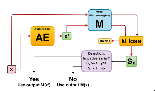
An adversarial score \(S\) is computed. \(S\) equals the K-L divergence between the model predictions on \(x\) and \(x'\).
If \(S\) is above a threshold (explicitly defined or inferred from training data), the instance is flagged as adversarial.
For adversarial instances, the model \(M\) uses the reconstructed instance \(x'\) to make a prediction. If the adversarial score is below the threshold, the model makes a prediction on the original instance \(x\).
This procedure is illustrated in the diagram below:
The method is very flexible and can also be used to detect common data corruptions and perturbations which negatively impact the model performance. The algorithm works well on tabular and image data.
Usage
Initialize
Parameters:
threshold: threshold value above which the instance is flagged as an adversarial instance.encoder_net:tf.keras.Sequentialinstance containing the encoder network. Example:
encoder_net = tf.keras.Sequential(
    [
        InputLayer(input_shape=(32, 32, 3)),
        Conv2D(32, 4, strides=2, padding='same',
               activation=tf.nn.relu, kernel_regularizer=l1(1e-5)),
        Conv2D(64, 4, strides=2, padding='same',
               activation=tf.nn.relu, kernel_regularizer=l1(1e-5)),
        Conv2D(256, 4, strides=2, padding='same',
               activation=tf.nn.relu, kernel_regularizer=l1(1e-5)),
        Flatten(),
        Dense(40)
    ]
)
decoder_net:tf.keras.Sequentialinstance containing the decoder network. Example:
decoder_net = tf.keras.Sequential(
[
        InputLayer(input_shape=(40,)),
        Dense(4 * 4 * 128, activation=tf.nn.relu),
        Reshape(target_shape=(4, 4, 128)),
        Conv2DTranspose(256, 4, strides=2, padding='same',
                        activation=tf.nn.relu, kernel_regularizer=l1(1e-5)),
        Conv2DTranspose(64, 4, strides=2, padding='same',
                        activation=tf.nn.relu, kernel_regularizer=l1(1e-5)),
        Conv2DTranspose(3, 4, strides=2, padding='same',
                        activation=None, kernel_regularizer=l1(1e-5))
    ]
)
ae: instead of using a separate encoder and decoder, the AE can also be passed as atf.keras.Model.model: the classifier as atf.keras.Model. Example:
inputs = tf.keras.Input(shape=(input_dim,))
outputs = tf.keras.layers.Dense(output_dim, activation=tf.nn.softmax)(inputs)
model = tf.keras.Model(inputs=inputs, outputs=outputs)
hidden_layer_kld: dictionary with as keys the number of the hidden layer(s) in the classification model which are extracted and used during training of the adversarial AE, and as values the output dimension for the hidden layer. Extending the training methodology to the hidden layers is optional and can further improve the adversarial correction mechanism.model_hl: instead of passing a dictionary tohidden_layer_kld, a list with tf.keras models for the hidden layer K-L divergence computation can be passed directly.w_model_hl: Weights assigned to the loss of each model inmodel_hl. Also used to weight the K-L divergence contribution for each model inmodel_hlwhen computing the adversarial score.temperature: Temperature used for model prediction scaling. Temperature <1 sharpens the prediction probability distribution which can be beneficial for prediction distributions with high entropy.data_type: can specify data type added to metadata. E.g. ‘tabular’ or ‘image’.
Initialized adversarial detector example:
from alibi_detect.ad import AdversarialAE

ad = AdversarialAE(
    encoder_net=encoder_net,
    decoder_net=decoder_net,
    model=model,
    temperature=0.5
)
Fit
We then need to train the adversarial detector. The following parameters can be specified:
X: training batch as a numpy array.loss_fn: loss function used for training. Defaults to the custom adversarial loss.w_model: weight on the loss term minimizing the K-L divergence between model prediction probabilities on the original and reconstructed instance. Defaults to 1.w_recon: weight on the mean squared error reconstruction loss term. Defaults to 0.optimizer: optimizer used for training. Defaults to Adam with learning rate 1e-3.epochs: number of training epochs.batch_size: batch size used during training.verbose: boolean whether to print training progress.log_metric: additional metrics whose progress will be displayed if verbose equals True.preprocess_fn: optional data preprocessing function applied per batch during training.
ad.fit(X_train, epochs=50)
The threshold for the adversarial score can be set via infer_threshold. We need to pass a batch of instances \(X\) and specify what percentage of those we consider to be normal via threshold_perc. Even if we only have normal instances in the batch, it might be best to set the threshold value a bit lower (e.g. \(95\)%) since the the model could have misclassified training instances leading to a higher score if the reconstruction picked up features from the correct class or some
instances might look adversarial in the first place.
ad.infer_threshold(X_train, threshold_perc=95, batch_size=64)
Detect
We detect adversarial instances by simply calling predict on a batch of instances X. We can also return the instance level adversarial score by setting return_instance_score to True.
The prediction takes the form of a dictionary with meta and data keys. meta contains the detector’s metadata while data is also a dictionary which contains the actual predictions stored in the following keys:
is_adversarial: boolean whether instances are above the threshold and therefore adversarial instances. The array is of shape (batch size,).instance_score: contains instance level scores ifreturn_instance_scoreequals True.
preds_detect = ad.predict(X, batch_size=64, return_instance_score=True)
Correct
We can immediately apply the procedure sketched out in the above diagram via correct. The method also returns a dictionary with meta and data keys. On top of the information returned by detect, 3 additional fields are returned under data:
corrected: model predictions by following the adversarial detection and correction procedure.no_defense: model predictions without the adversarial correction.defense: model predictions where each instance is corrected by the defense, regardless of the adversarial score.
preds_correct = ad.correct(X, batch_size=64, return_instance_score=True)