Background
1. What is drift?
Although powerful, modern machine learning models can be sensitive. Seemingly subtle changes in a data distribution can destroy the performance of otherwise state-of-the art models, which can be especially problematic when ML models are deployed in production. Typically, ML models are tested on held out data in order to estimate their future performance. Crucially, this assumes that the process underlying the input data \(\mathbf{X}\) and output data \(\mathbf{Y}\) remains constant.
Drift is said to occur when the process underlying \(\mathbf{X}\) and \(\mathbf{Y}\) at test time differs from the process that generated the training data. In this case, we can no longer expect the model’s performance on test data to match that observed on held out training data. At test time we always observe features \(\mathbf{X}\), and the ground truth then refers to a corresponding label \(\mathbf{Y}\). If ground truths are available at test time, supervised drift detection can be performed, with the model’s predictive performance monitored directly. However, in many scenarios, such as the binary classification example below, ground truths are not available and unsupervised drift detection methods are required.
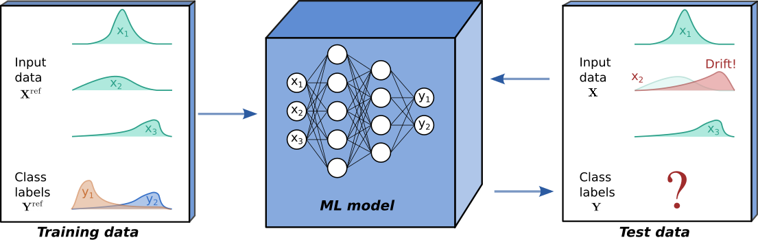
To explore the different types of drift, consider the common scenario where we deploy a model \(f: \boldsymbol{x} \mapsto y\) on input data \(\mathbf{X}\) and output data \(\mathbf{Y}\), jointly distributed according to \(P(\mathbf{X},\mathbf{Y})\). The model is trained on training data drawn from a distribution \(P_{ref}(\mathbf{X},\mathbf{Y})\). Drift is said to have occurred when \(P(\mathbf{X},\mathbf{Y}) \ne P_{ref}(\mathbf{X},\mathbf{Y})\). Writing the joint distribution as
we can classify drift under a number of types:
Covariate drift: Also referred to as input drift, this occurs when the distribution of the input data has shifted \(P(\mathbf{X}) \ne P_{ref}(\mathbf{X})\), whilst \(P(\mathbf{Y}|\mathbf{X})\) = \(P_{ref}(\mathbf{Y}|\mathbf{X})\). This may result in the model giving unreliable predictions.
Prior drift: Also referred to as label drift, this occurs when the distribution of the outputs has shifted \(P(\mathbf{Y}) \ne P_{ref}(\mathbf{Y})\), whilst \(P(\mathbf{X}|\mathbf{Y})=P_{ref}(\mathbf{X}|\mathbf{Y})\). This can affect the model’s decision boundary, as well as the model’s performance metrics.
Concept drift: This occurs when the process generating \(y\) from \(x\) has changed, such that \(P(\mathbf{Y}|\mathbf{X}) \ne P_{ref}(\mathbf{Y}|\mathbf{X})\). It is possible that the model might no longer give a suitable approximation of the true process.
Note that a change in one of the conditional probabilities \(P(\mathbf{X}|\mathbf{Y})\) and \(P(\mathbf{Y}|\mathbf{X})\) does not necessarily imply a change in the other. For example, consider the pneumonia prediction example from Lipton et al., whereby a classification model \(f\) is trained to predict \(y\), the occurrence (or not) of pneumonia, given a list of symptoms \(\boldsymbol{x}\). During a pneumonia outbreak, \(P(\mathbf{Y}|\mathbf{X})\) (e.g. pneumonia given cough) might rise, but the manifestations of the disease \(P(\mathbf{X}|\mathbf{Y})\) might not change. In many cases, knowledge of underlying causal structure of the problem can be used to deduce that one of the conditionals will remain unchanged.
Below, the different types of drift are visualised for a simple two-dimensional classification problem. It is possible for a drift to fall under more than one category, for example the prior drift below also happens to be a case of covariate drift.
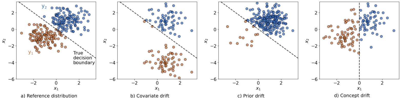
It is relatively easy to spot drift by eyeballing these figures here.
However, the task becomes considerably harder for high-dimensional real
problems, especially since real-time ground truths are not typically
available. Some types of drift, such as prior and concept drift, are
especially difficult to detect without access to ground truths. As a
workaround proxies are required, for example a model’s predictions can
be monitored to check for prior drift.
2. Detecting drift
Alibi Detect offers a wide array of methods for detecting drift (see here), some of which are examined in the NeurIPS 2019 paper Failing Loudly: An Empirical Study of Methods for Detecting Dataset Shift. Generally, these aim to determine whether the distribution \(P(\mathbf{z})\) has drifted from a reference distribution \(P_{ref}(\mathbf{z})\), where \(\mathbf{z}\) may represent input data \(\mathbf{X}\), true output data \(\mathbf{Y}\), or some form of model output, depending on what type of drift we wish to detect.
Due to natural randomness in the process being modelled, we don’t necessarily expect observations \(\mathbf{z}_1,\dots,\mathbf{z}_N\) drawn from \(P(\mathbf{z})\) to be identical to \(\mathbf{z}^{ref}_1,\dots,\mathbf{z}^{ref}_M\) drawn from \(P_{ref}(\mathbf{z})\). To decide whether differences between \(P(\mathbf{z})\) and \(P_{ref}(\mathbf{z})\) are due to drift or just natural randomness in the data, statistical two-sample hypothesis testing is used, with the null hypothesis \(P(\mathbf{z})=P_{ref}(\mathbf{z})\). If the \(p\)-value obtained is below a given threshold, the null is rejected and the alternative hypothesis \(P(\mathbf{z}) \ne P_{ref}(\mathbf{z})\) is accepted, suggesting drift is occurring.
Since \(\mathbf{z}\) is often high-dimensional (even a 200 x 200 greyscale image has 40k dimensions!), performing hypothesis testing in the full-space is often either computationally intractable, or unsuitable for the chosen statistical test. Instead, the pipeline below is often used, with dimension reduction as a pre-processing step.
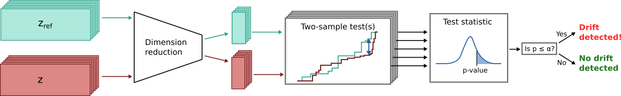
Figure inspired by Figure 1 in Failing Loudly: An Empirical Study of Methods for Detecting Dataset Shift.
Hypothesis testing
Hypothesis testing involves first choosing a test statistic \(S(\mathbf{z})\), which is expected to be small if the null hypothesis \(H_0\) is true, and large if the alternative \(H_a\) is true. For observed data \(\mathbf{z}\), \(S(\mathbf{z})\) is computed, followed by a \(p\)-value \(\hat{p} = P(\text{such an extreme } S(\mathbf{z}) | H_0)\). In other words, \(\hat{p}\) represents the probability of such an extreme value of \(S(\mathbf{z})\) occurring given that \(H_0\) is true. When \(\hat{p}\le \alpha\), results are said to be statistically significant, and the null \(P(\mathbf{z})=P_{ref}(\mathbf{z})\) is rejected. Conveniently, the threshold \(\alpha\) represents the desired false positive rate.
The test statistics available in Alibi Detect can be broadly split into two categories; univariate and multivariate tests:
Univariate:
Chi-Squared (for categorical data)
Fisher’s Exact Test (for binary data)
Multivariate:
When applied to multidimensional data with dimension \(d\), the univariate tests are applied in a feature-wise manner. The obtained \(p\)-values for each feature are aggregated either via the Bonferroni or the False Discovery Rate (FDR) correction. The Bonferroni correction is more conservative and controls for the probability of at least one false positive. The FDR correction on the other hand allows for an expected fraction of false positives to occur. If the tests (i.e. each feature dimension) are independent, these corrections preserve the desired false positive rate (FPR). However, usually this is not the case, resulting in FPR’s up to \(d\)-times lower than desired, which becomes especially problematic when \(d\) is large. Additionally, since the univariate tests examine the feature-wise marginal distributions, they may miss drift in cases where the joint distribution over all \(d\) features has changed, but the marginals have not. The multivariate tests avoid these problems, at the cost of greater complexity.
Dimension reduction
Given an input dataset \(\mathbf{X}\in \mathbb{R}^{N\times d}\), where \(N\) is the number of observations and \(d\) the number of dimensions, the aim is to reduce the data dimensionality from \(d\) to \(K\), where \(K\ll d\). A drift detector can then be applied to the lower dimensional data \(\hat{\mathbf{X}}\in \mathbb{R}^{N\times K}\), where distances more meaningfully capture notions of similarity/dissimilarity between instances. Dimension reduction approaches can be broadly categorised under:
Linear projections
Non-linear projections
Feature maps (from ML model)
Model uncertainty
Alibi Detect allows for a
high degree of flexibility here, with a user’s chosen dimension
reduction technique able to be incorporated into their chosen detector
via the preprocess_fn argument (and sometimes
preprocess_batch_fn and preprocess_at_init, depending on the
detector). In the following sections, the three categories of techniques
are briefly introduced. Alibi Detect offers the following functionality
using either TensorFlow or
PyTorch backends and preprocessing utilities.
For more details, see the examples.
Linear projections
This includes dimension reduction techniques such as principal
component analysis
(PCA)
and sparse random projections
(SRP). These techniques
involve using a transformation or projection matrix \(\mathbf{R}\)
to reduce the dimensionality of a given data matrix \(\mathbf{X}\),
such that \(\hat{\mathbf{X}} = \mathbf{XR}\). A straightforward way
to include such techniques as a pre-processing stage is to pass them to
the detectors via the preprocess_fn argument, for example for the
scikit-learn library’s PCA class:
pca = PCA(2)
pca.fit(X_train)
detector = MMDDrift(X_ref, backend='tensorflow', p_val=.05, preprocess_fn=pca.transform)
Note 1: Disjoint training and reference data sets
Astute readers may have noticed that in the code snippet above,
the data X_train is used to “train” the PCA model, but
the MMDDrift detector is initialised with X_ref. This is a
subtle yet important point. If a detector’s preprocessor (a
dimension reduction or other input
preprocessing step) is trained on the
reference data (X_ref), any over-fitting to this data may make
the resulting detector overly sensitive to differences between the
reference and test data sets.
To avoid an overly discriminative detector, it is customary to draw two disjoint datasets from \(P_{ref}(\mathbf{z})\), a training set and a held-out reference set. The training data is used to train any input preprocessing steps, and the detector is then initialised on the reference set, and used to detect drift between the reference and test set. This also applies to the learned drift detectors, which should be trained on the training set not the reference set.
Non-linear projections
A common strategy for obtaining non-linear dimension reducing
representations is to use an autoencoder, but other non-linear
techniques
can also be used. Autoencoders consist of an encoder function
\(\phi : \mathcal{X} \mapsto \mathcal{H}\) and a decoder function
\(\psi : \mathcal{H} \mapsto \mathcal{X}\), where the latent space
\(\mathcal{H}\) has lower dimensionality than the input space
\(\mathcal{X}\). The output of the encoder
\(\hat{\mathbf{X}} \in \mathcal{H}\) can then be monitored by the
drift detector. Training involves learning both the encoding function
\(\phi\) and the decoding function \(\psi\), in order to reduce
the reconstruction loss, e.g. if MSE is used:
\(\phi, \psi = \text{arg} \min_{\phi, \psi}\, \lVert \mathbf{X}-(\phi \circ \psi)\mathbf{X}\rVert^2\).
However, untrained (randomly initialised) autoencoders can also be used.
For an example, a pytorch autoencoder can be incorporated into a
detector by packaging it as a callable function using preprocess_drift()
and partial():
encoder_net = torch.nn.Sequential(...)
preprocess_fn = partial(preprocess_drift, model=encoder_net, batch_size=512)
detector = MMDDrift(X_ref, backend='pytorch', p_val=.05, preprocess_fn=preprocess_fn)
Feature maps
Following Detecting and Correcting for Label Shift with Black Box Predictors, feature maps can be extracted from existing pre-trained black-box models such as the image classifier shown below. Instead of using the latent space as the dimensionality-reducing representation, other layers of the model such as the softmax outputs or predicted class-labels can also be extracted and monitored. Since different layers yield different output dimensions, different hypothesis tests are required for each.
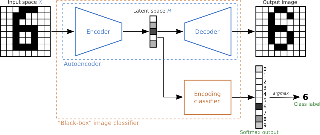
Figure inspired by this MNIST classification example from the timeserio package.
Failing Loudly: An Empirical Study of Methods for Detecting Dataset
Shift shows that extracting
feature maps from existing models can be an effective technique, which
is encouraging since this allows the user to repurpose existing
black-box models for use as drift detectors. The syntax for
incorporating existing models into drift detectors is similar to the
previous autoencoder example, with the added step of using
HiddenOutput
to select the model’s network layer to extract outputs from. The code
snippet below is borrowed from Maximum Mean Discrepancy drift detector
on CIFAR-10, where the softmax
layer of the well-known
ResNet-32 model is fed into
an MMDDrift detector.
clf = fetch_tf_model('cifar10', 'resnet32')
preprocess_fn = partial(preprocess_drift, model=HiddenOutput(clf, layer=-1), batch_size=128)
detector = MMDDrift(X_ref, backend='tensorflow', p_val=.05,preprocess_fn=preprocess_fn)
Model uncertainty
The model uncertainty-based drift detector uses the ML model of interest itself to detect drift. These detectors aim to directly detect drift that’s likely to affect the performance of a model of interest. The approach is to test for change in the number of instances falling into regions of the input space on which the model is uncertain in its predictions. For each instance in the reference set the detector obtains the model’s prediction and some associated notion of uncertainty. The same is done for the test set and if significant differences in uncertainty are detected (via a Kolmogorov-Smirnoff test) then drift is flagged. The model’s notion of uncertainty depends on the type of model. For a classifier this may be the entropy of the predicted label probabilities. For a regressor with dropout layers, dropout Monte Carlo can be used to provide a notion of uncertainty.
The model uncertainty-based detectors are classed under the dimension
reduction category since a model’s uncertainty is by definition one-dimensional.
However, the syntax for the uncertainty-based detectors is different to the
other detectors. Instead of passing a pre-processing step to a detector via
a preprocess_fn (or similar) argument, the dimension reduction (in this case
computing a notion of uncertainty) is performed internally by these detectors.
reg =  # pytorch regression model with at least 1 dropout layer
detector = RegressorUncertaintyDrift(x_ref, reg, backend='pytorch',
                                     p_val=.05, uncertainty_type='mc_dropout')
Input preprocessing
Dimension reduction is a common preprocessing task (e.g. for covariate drift detection on tabular or image data), but some modalities of data (e.g. text and graph data) require other forms of preprocessing in order for drift detection to be performed effectively.
Text data
When dealing with text data, performing drift detection on raw strings or tokenized data is not effective since they don’t represent the semantics of the input. Instead, we extract contextual embeddings from language transformer models and detect drift on those. This procedure has a significant impact on the type of drift we detect. Strictly speaking we are not detecting covariate/input drift anymore since the entire training procedure (objective function, training data etc) for the (pre)trained embeddings has an impact on the embeddings we extract.
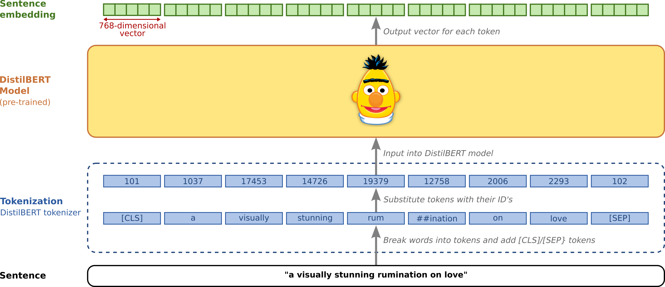
Figure based on Jay Alammar’s excellent visual guide to the BERT model
Alibi Detect contains functionality to leverage pre-trained embeddings
from HuggingFace’s
transformer package. Popular
models such as BERT or
DistilBERT (shown above) can be
used, but Alibi Detect also allows you to easily use your own embeddings
of choice. A subsequent dimension reduction step can also be applied if
necessary, as is done in the Text drift detection on IMDB movie
reviews example, where the
768-dimensional embeddings from the BERT model are passed through an
untrained AutoEncoder to reduce their dimensionality. Alibi Detect
allows various types of embeddings to be extracted from transformer
models, using TransformerEmbedding.
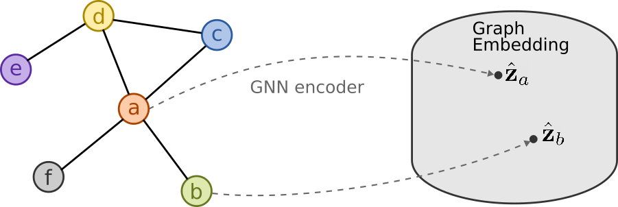
Graph data
In a similar manner to text data, graph data requires preprocessing before drift detection can be performed. This can be done by extracting graph embeddings from graph neural network (GNN) encoders, as shown below, and demonstrated in the Drift detection on molecular graphs example.
Simple example
For a simple example, we’ll use the MMD detector to check for drift on the two-dimensional binary classification problem shown previously (see notebook). The MMD detector is a kernel-based method for multivariate two sample testing. Since the number of dimensions is already low, dimension reduction step is not necessary here here. For a more advanced example using the MMD detector with dimension reduction, check out the Maximum Mean Discrepancy drift detector on CIFAR-10 example.
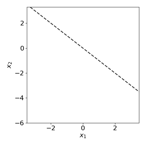
The true model/process is defined as:
where the slope \(s\) is set as \(s=-1\).
def true_model(X,slope=-1):
    z = slope*X[:,0]
    idx = np.argwhere(X[:,1]>z)
    y = np.zeros(X.shape[0])
    y[idx] = 1
    return y

true_slope = -1
The reference distribution is defined as a mixture of two Normal distributions:
with the standard deviation set at \(\sigma=0.8\), and the weights
set to \(\phi_1=\phi_2=0.5\). Reference data \(\mathbf{X}^{ref}\) and training
data \(\mathbf{X}^{train}\) (see Note 1) can be generated by sampling from
this distribution. The corresponding labels \(\mathbf{Y}^{ref}\) and \(\mathbf{Y}^{train}\) are obtained
by evaluating true_model().
# Reference distribution
sigma = 0.8
phi1 = 0.5
phi2 = 0.5
ref_norm_0 = multivariate_normal([-1,-1], np.eye(2)*sigma**2)
ref_norm_1 = multivariate_normal([ 1, 1], np.eye(2)*sigma**2)

# Reference data (to initialise the detectors)
N_ref = 240
X_0 = ref_norm_0.rvs(size=int(N_ref*phi1),random_state=1)
X_1 = ref_norm_1.rvs(size=int(N_ref*phi2),random_state=1)
X_ref = np.vstack([X_0, X_1])
y_ref = true_model(X_ref,true_slope)

# Training data (to train the classifer)
N_train = 240
X_0 = ref_norm_0.rvs(size=int(N_train*phi1),random_state=0)
X_1 = ref_norm_1.rvs(size=int(N_train*phi2),random_state=0)
X_train = np.vstack([X_0, X_1])
y_train = true_model(X_train,true_slope)
For a model, we choose the well-known decision tree classifier. As well as training the model, this is a good time to initialise the MMD detector with the held-out reference data \(\mathbf{X}^{ref}\) by calling:
detector = MMDDrift(X_ref, backend='pytorch', p_val=.05)
The significance threshold is set at \(\alpha=0.05\), meaning the detector will flag results as drift detected when the computed \(p\)-value is less than this i.e. \(\hat{p}< \alpha\).
# Fit decision tree classifier
from sklearn.tree import DecisionTreeClassifier
clf = DecisionTreeClassifier(max_depth=20)
clf.fit(X_train, y_train)

# Plot with a pre-defined helper function
plot(X_ref,y_ref,true_slope,clf=clf)

# Classifier accuracy
print('Mean training accuracy %.2f%%' %(100*clf.score(X_ref,y_ref)))

# Fit a drift detector to the training data
from alibi_detect.cd import MMDDrift
detector = MMDDrift(X_ref, backend='pytorch', p_val=.05)
Mean training accuracy 99.17%
No GPU detected, fall back on CPU.
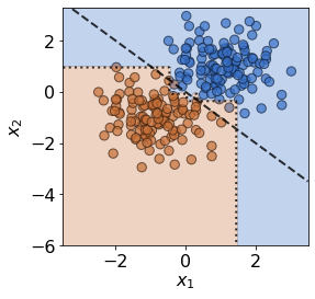
No drift
Before introducing drift, we first examine the case where no drift is present. We resample from the same mixture of Gaussian distributions to generate test data \(\mathbf{X}\). The individual data observations are different, but the underlying distributions are unchanged, hence no true drift is present.
N_test = 120
X_0 = ref_norm_0.rvs(size=int(N_test*phi1),random_state=2)
X_1 = ref_norm_1.rvs(size=int(N_test*phi2),random_state=2)
X_test = np.vstack([X_0, X_1])

# Plot
y_test = true_model(X_test,true_slope)
plot(X_test,y_test,true_slope,clf=clf)

# Classifier accuracy
print('Mean test accuracy %.2f%%' %(100*clf.score(X_test,y_test)))
Mean test accuracy 95.00%
Unsurprisingly, the model’s mean test accuracy is relatively high. To
run the detector on test data the .predict() is used:
detector.predict(X_test)
{'data': {'is_drift': 0,
  'distance': 0.0023595122654528344,
  'p_val': 0.30000001192092896,
  'threshold': 0.05,
  'distance_threshold': 0.008109889},
 'meta': {'name': 'MMDDriftTorch',
  'detector_type': 'offline',
  'data_type': None,
  'backend': 'pytorch'}}
For the test statistic \(S(\mathbf{X})\) (we write \(S(\mathbf{X})\) instead of \(S(\mathbf{z})\) since the detector is operating on input data), the MMD detector uses the kernel trick to compute unbiased estimates of \(\text{MMD}^2\). The \(\text{MMD}\) is a distance-based measure between the two distributions \(P\) and \(P_{ref}\), based on the mean embeddings \(\mu\) and \(\mu_{ref}\) in a reproducing kernel Hilbert space \(F\):
A \(p\)-value is then obtained via a permutation
test on the
estimates of \(\text{MMD}^2\). As expected, since we are sampling from
the reference distribution \(P_{ref}(\mathbf{X})\), the detector’s
prediction is 'is_drift':0 here, indicating that drift is not
detected. More specifically, the detector’s \(p\)-value (p_val)
is above the threshold of \(\alpha=0.05\) (threshold),
indicating that no statistically significant drift has been detected.
The .predict() method also returns \(\hat{S}(\mathbf{X})\)
(distance_threshold), which is the threshold in terms of the test
statistic \(S(\mathbf{X})\) i.e. when
\(S(\mathbf{X})\ge \hat{S}(\mathbf{X})\) statistically significant
drift has been detected.
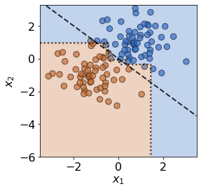
Covariate and prior drift
To impose covariate drift, we apply a shift to the mean of one of the normal distributions:
shift_norm_0 = multivariate_normal([2, -4], np.eye(2)*sigma**2)
X_0 = shift_norm_0.rvs(size=N_test*phi1,random_state=2)
X_1 = ref_norm_1.rvs(size=N_test*phi2,random_state=2)
X_test = np.vstack([X_0, X_1])

# Plot
y_test = true_model(X_test,slope)
plot(X_test,y_test,slope,clf=clf)

# Classifier accuracy
print('Mean test accuracy %.2f%%' %(100*clf.score(X_test,y_test)))

# Check for drift in covariates
pred = detector.predict(X_test)
labels = ['No','Yes']
print('Is drift? %s!' %labels[pred['data']['is_drift']])
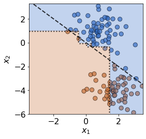
Mean test accuracy 66.67%
Is drift? Yes!
The test data has drifted into a previously unseen region of feature space, and the model is now misclassifying a number of test observations. If true test labels are available, this is easily detectable by monitoring the test accuracy. However, labels are not always available at test time, in which case a drift detector monitoring the covariates comes in handy. In this case, the MMD detector successfully detects the covariate drift.
In a similar manner, a proxy for prior drift can be monitored by initialising a detector on labels from the reference set, and then feeding it a model’s predicted labels:
label_detector = MMDDrift(y_ref.reshape(-1,1), backend='tensorflow', p_val=.05)
y_pred = clf.predict(X_test)
label_detector.predict(y_pred.reshape(-1,1))
3. Learned drift detection
It can often be challenging to specify a test statistic \(S(\mathbf{z})\) that is large when drift is present and small otherwise. Alibi Detect offers a number of learned detectors, which try to explicitly learn a test statistic which satisfies this property:
Spot-the-diff(erence)
These detectors can be highly effective, but require training hence potentially increasing data requirements and set-up time. Similarly to when training preprocessing steps, it is important that the learned detectors are trained on training data which is held-out from the reference data set (see Note 1). A brief overview of these detectors is given below. For more details, see the detectors’ respective pages.
Learned kernel
The MMD detector uses a kernel \(k(\mathbf{z},\mathbf{z}^{ref})\) to compute unbiased estimates of \(\text{MMD}^2\). The user is free to provide their own kernel, but by default a Gaussian RBF kernel is used. The Learned kernel drift detector (Liu et al., 2020) extends this approach by training a kernel to maximise an estimate of the resulting test power. The learned kernel is defined as
where \(\Phi\) is a learnable projection, \(k_a\) and \(k_b\) are simple characteristic kernels (such as a Gaussian RBF), and \(\epsilon>0\) is a small constant. By letting \(\Phi\) be very flexible we can learn powerful kernels in this manner.
The figure below compares the use of a Gaussian and a learned kernel for identifying differences between two distributions \(P\) and \(P_{ref}\). The distributions are each equal mixtures of nine Gaussians with the same modes, but each component of \(P_{ref}\) is an isotropic Gaussian, whereas the covariance of \(P\) differs in each component. The Gaussian kernel (c) treats points isotropically throughout the space, based upon \(\lVert \mathbf{z} - \mathbf{z}^{ref} \rVert\) only. The learned kernel (d) behaves differently in different regions of the space, adapting to local structure and therefore allowing better detection of differences between \(P\) and \(P_{ref}\).
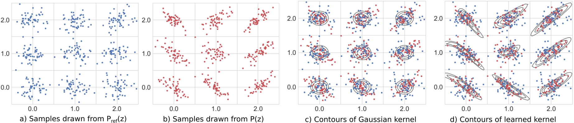
Original image source: Liu et al., 2020. Captions modified to match notation used elsewhere on this page.
Classifier
The classifier-based drift detector (Lopez-Paz and Oquab, 2017) attempts to detect drift by explicitly training a classifier to discriminate between data from the reference and test sets. The statistical test used depends on whether the classifier outputs probabilities or binarized (0 or 1) predictions, but the general idea is to determine whether the classifiers performance is statistically different from random chance. If the classifier can learn to discriminate better than randomly (in a generalisable manner) then drift must have occurred.
Liu et al. show that a classifier-based drift detector is actually a special case of the learned kernel. An important difference is that to train a classifier we maximise its accuracy (or a cross-entropy proxy), while for a learned kernel we maximise the test power directly. Liu et al. show that the latter approach is empirically superior.
Spot-the-diff
The spot-the-diff(erence) drift detector is an extension of the Classifier drift detector, where the classifier is specified in a manner that makes detections interpretable at the feature level when they occur. The detector is inspired by the work of Jitkrittum et al. (2016) but various major adaptations have been made.
As with the usual classifier-based approach, a portion of the available data is used to train a classifier that can discriminate reference instances from test instances. However, the spot-the-diff detector is specified such that when drift is detected, we can inspect the weights of the classifier to shine light on exactly which features of the data were used to distinguish reference from test samples, and therefore caused drift to be detected. The Interpretable drift detection with the spot-the-diff detector on MNIST and Wine-Quality datasets example demonstrates this capability.
4. Online drift detection
So far, we have discussed drift detection in an offline context, with the entire test set \(\{\mathbf{z}_i\}_{i=1}^{N}\) compared to the reference dataset \(\{\mathbf{z}^{ref}_i\}_{i=1}^{M}\). However, at test time, data sometimes arrives sequentially. Here it is desirable to detect drift in an online fashion, allowing us to respond as quickly as possible and limit the damage it might cause.
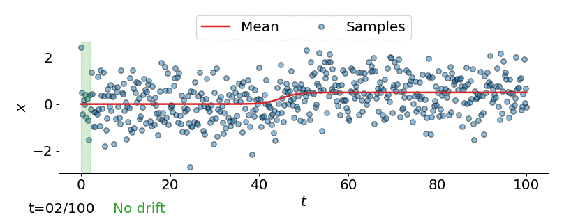
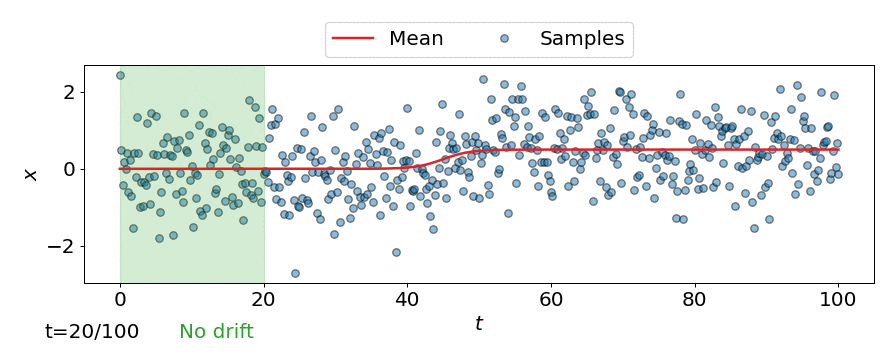
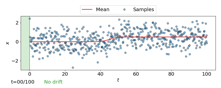
One approach is to perform a test for drift every \(W\) time-steps, using the \(W\) samples that have arrived since the last test. In other words, that is to compare \(\{\mathbf{z}_i\}_{i=t-W+1}^{t}\) to \(\{\mathbf{z}^{ref}_i\}_{i=1}^{M}\). Such a strategy could be implemented using any of the offline detectors implemented in alibi-detect, but being both sensitive to slight drift and responsive to severe drift is difficult. If the window size \(W\) is too large the delay between consecutive statistical tests hampers responsiveness to severe drift, but an overly small window is unreliable. This is demonstrated below, where the offline MMD detector is used to monitor drift in data \(\mathbf{X}\) sampled from a normal distribution \(\mathcal{N}\left(\mu,\sigma^2 \right)\) over time \(t\), with the mean starting to drift from \(\mu=0\) to \(\mu=0.5\) at \(t=40\).
Online drift detectors
An alternative strategy is to perform a test each time data arrives. However the usual offline methods are not applicable because the process for computing \(p\)-values is too expensive. Additionally, they don’t account for correlated test outcomes when using overlapping windows of test data, leading to miscalibrated detectors operating at an unknown False Positive Rate (FPR). Well-calibrated FPR’s are crucial for judging the significance of a drift detection. In the absence of calibration, drift detection can be useless since there is no way of knowing what fraction of detections are false positives. To tackle this problem, Alibi Detect offers specialist online drift detectors:
These detectors leverage the calibration method introduced by Cobb et al. (2021) in order to ensure they are well well-calibrated when used in a sequential manner. The detectors compute a test statistic \(S(\mathbf{z})\) during the configuration phase. Then, at test time, the test statistic is updated sequentially at a low cost. When no drift has occurred the test statistic fluctuates around its expected value, and once drift occurs the test statistic starts to drift upwards. When it exceeds some preconfigured threshold value, drift is detected. The online detectors are constructed in a similar manner to the offline detectors, for example for the online MMD detector:
online_detector = MMDDriftOnline(X_ref, ert, window_size, backend='tensorflow', n_bootstraps=5000)
But, in addition to providing the detector with reference data, the expected run-time (see below), and size of the sliding window must also be defined. Another important difference is that the online detectors make predictions on single data instances:
result = online_detector.predict(X[i])
This can be seen in the animation below, where the online detector considers each incoming observation/sample individually, instead of considering a batch of observations like the offline detectors.
Expected run-time and detection delay
Unlike offline detectors which require the specification of a threshold \(p\)-value, which is equivalent to a false positive rate (FPR), the online detectors in alibi-detect require the specification of an expected run-time (ERT) (an inverted FPR). This is the number of time-steps that we insist our detectors, on average, should run for in the absence of drift, before making a false detection.
Usually we would like the ERT to be large, however this results in
insensitive detectors which are slow to respond when drift does occur.
Hence, there is a tradeoff between the expected run time and the
expected detection delay (the time taken for the detector to respond to
drift in the data). To target the desired ERT, thresholds are configured
during an initial configuration phase via simulation (n_bootstraps
sets the number of boostrap simulations used here). This configuration
process is only suitable when the amount of reference data is relatively
large (ideally around an order of magnitude larger than the desired
ERT). Configuration can be expensive (less so with a GPU), but allows
the detector to operate at a low-cost at test time. For a more in-depth
explanation, see Drift Detection: An Introduction with
Seldon.