This page was generated from examples/cd_clf_cifar10.ipynb.

Learned drift detectors on CIFAR-10

Under the hood drift detectors leverage a function (also known as a test-statistic) that is expected to take a large value if drift has occurred and a low value if not. The power of the detector is partly determined by how well the function satisfies this property. However, specifying such a function in advance can be very difficult. In this example notebook we consider two ways in which a portion of the available data may be used to learn such a function before then applying it on the held out portion of the data to test for drift.

Detecting drift with a learned classifier

The classifier-based drift detector simply tries to correctly distinguish instances from the reference data vs. the test set. The classifier is trained to output the probability that a given instance belongs to the test set. If the probabilities it assigns to unseen tests instances are significantly higher (as determined by a Kolmogorov-Smirnov test) to those it assigns to unseen reference instances then the test set must differ from the reference set and drift is flagged. To leverage all the available reference and test data, stratified cross-validation can be applied and the out-of-fold predictions are used for the significance test. Note that a new classifier is trained for each test set or even each fold within the test set.

Backend

The method works with both the PyTorch and TensorFlow frameworks. Alibi Detect does however not install PyTorch for you. Check the PyTorch docs how to do this.

Dataset

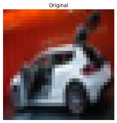
CIFAR10 consists of 60,000 32 by 32 RGB images equally distributed over 10 classes. We evaluate the drift detector on the CIFAR-10-C dataset (Hendrycks & Dietterich, 2019). The instances in CIFAR-10-C have been corrupted and perturbed by various types of noise, blur, brightness etc. at different levels of severity, leading to a gradual decline in the classification model performance. We also check for drift against the original test set with class imbalances.

import matplotlib.pyplot as plt
import numpy as np
import tensorflow as tf

from alibi_detect.cd import ClassifierDrift
from alibi_detect.datasets import fetch_cifar10c, corruption_types_cifar10c

Load data

Original CIFAR-10 data:

(X_train, y_train), (X_test, y_test) = tf.keras.datasets.cifar10.load_data()
X_train = X_train.astype('float32') / 255
X_test = X_test.astype('float32') / 255
y_train = y_train.astype('int64').reshape(-1,)
y_test = y_test.astype('int64').reshape(-1,)

For CIFAR-10-C, we can select from the following corruption types at 5 severity levels:

corruptions = corruption_types_cifar10c()
print(corruptions)

['brightness', 'contrast', 'defocus_blur', 'elastic_transform', 'fog', 'frost', 'gaussian_blur', 'gaussian_noise', 'glass_blur', 'impulse_noise', 'jpeg_compression', 'motion_blur', 'pixelate', 'saturate', 'shot_noise', 'snow', 'spatter', 'speckle_noise', 'zoom_blur']

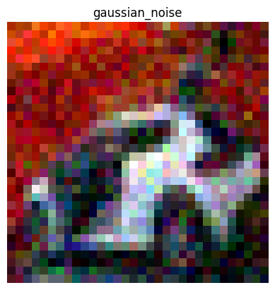
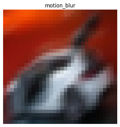
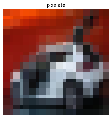
Let’s pick a subset of the corruptions at corruption level 5. Each corruption type consists of perturbations on all of the original test set images.

corruption = ['gaussian_noise', 'motion_blur', 'brightness', 'pixelate']
X_corr, y_corr = fetch_cifar10c(corruption=corruption, severity=5, return_X_y=True)
X_corr = X_corr.astype('float32') / 255

We split the original test set in a reference dataset and a dataset which should not be flagged as drift. We also split the corrupted data by corruption type:

np.random.seed(0)
n_test = X_test.shape[0]
idx = np.random.choice(n_test, size=n_test // 2, replace=False)
idx_h0 = np.delete(np.arange(n_test), idx, axis=0)
X_ref,y_ref = X_test[idx], y_test[idx]
X_h0, y_h0 = X_test[idx_h0], y_test[idx_h0]
print(X_ref.shape, X_h0.shape)

(5000, 32, 32, 3) (5000, 32, 32, 3)

n_corr = len(corruption)
X_c = [X_corr[i * n_test:(i + 1) * n_test] for i in range(n_corr)]

We can visualise the same instance for each corruption type:

i = 6

n_test = X_test.shape[0]
plt.title('Original')
plt.axis('off')
plt.imshow(X_test[i])
plt.show()
for _ in range(len(corruption)):
    plt.title(corruption[_])
    plt.axis('off')
    plt.imshow(X_corr[n_test * _+ i])
    plt.show()

Detect drift with a TensorFlow classifier

Single fold

We use a simple classification model and try to distinguish between the reference data and the corrupted test sets. The detector defaults to binarize=False which means a Kolmogorov-Smirnov test will be used to test for significant disparity between continuous model predictions (e.g. probabilities or logits). Initially we’ll test at a significance level of \(p=0.05\), use \(75\)% of the shuffled reference and test data for training and evaluate the detector on the remaining \(25\)%. We only train for 1 epoch.

from tensorflow.keras.layers import Conv2D, Dense, Flatten, Input

tf.random.set_seed(0)

model = tf.keras.Sequential(
  [
      Input(shape=(32, 32, 3)),
      Conv2D(8, 4, strides=2, padding='same', activation=tf.nn.relu),
      Conv2D(16, 4, strides=2, padding='same', activation=tf.nn.relu),
      Conv2D(32, 4, strides=2, padding='same', activation=tf.nn.relu),
      Flatten(),
      Dense(2, activation='softmax')
  ]
)

cd = ClassifierDrift(X_ref, model, p_val=.05, train_size=.75, epochs=1)

If needed, the detector can be saved and loaded with save_detector and load_detector:

from alibi_detect.saving import save_detector, load_detector
# Save detector
filepath = 'tf_detector'
save_detector(cd, filepath)

# Load detector
cd = load_detector(filepath)

WARNING:tensorflow:Compiled the loaded model, but the compiled metrics have yet to be built. `model.compile_metrics` will be empty until you train or evaluate the model.
WARNING:tensorflow:No training configuration found in the save file, so the model was *not* compiled. Compile it manually.

Let’s check whether the detector thinks drift occurred on the different test sets and time the prediction calls:

from timeit import default_timer as timer

labels = ['No!', 'Yes!']

def make_predictions(cd, x_h0, x_corr, corruption):
    t = timer()
    preds = cd.predict(x_h0)
    dt = timer() - t
    print('No corruption')
    print('Drift? {}'.format(labels[preds['data']['is_drift']]))
    print(f'p-value: {preds["data"]["p_val"]:.3f}')
    print(f'Time (s) {dt:.3f}')

    if isinstance(x_corr, list):
        for x, c in zip(x_corr, corruption):
            t = timer()
            preds = cd.predict(x)
            dt = timer() - t
            print('')
            print(f'Corruption type: {c}')
            print('Drift? {}'.format(labels[preds['data']['is_drift']]))
            print(f'p-value: {preds["data"]["p_val"]:.3f}')
            print(f'Time (s) {dt:.3f}')

make_predictions(cd, X_h0, X_c, corruption)

No corruption
Drift? No!
p-value: 0.963
Time (s) 3.412

Corruption type: gaussian_noise
Drift? Yes!
p-value: 0.000
Time (s) 3.194

Corruption type: motion_blur
Drift? Yes!
p-value: 0.000
Time (s) 3.233

Corruption type: brightness
Drift? Yes!
p-value: 0.000
Time (s) 3.162

Corruption type: pixelate
Drift? Yes!
p-value: 0.000
Time (s) 3.210

As expected, drift was only detected on the corrupted datasets and the classifier could easily distinguish the corrupted from the reference data.

Use all the available data via cross-validation

So far we’ve only used \(25\)% of the data to detect the drift since \(75\)% is used for training purposes. At the cost of additional training time we can however leverage all the data via stratified cross-validation. We just need to set the number of folds and keep everything else the same. So for each test set n_folds models are trained, and the out-of-fold predictions combined for the significance test:

cd = ClassifierDrift(X_ref, model, p_val=.05, n_folds=5, epochs=1)

Both `n_folds` and `train_size` specified. By default `n_folds` is used.

make_predictions(cd, X_h0, X_c, corruption)

No corruption
Drift? No!
p-value: 0.738
Time (s) 11.437

Corruption type: gaussian_noise
Drift? Yes!
p-value: 0.000
Time (s) 16.781

Corruption type: motion_blur
Drift? Yes!
p-value: 0.000
Time (s) 19.431

Corruption type: brightness
Drift? Yes!
p-value: 0.000
Time (s) 17.203

Corruption type: pixelate
Drift? Yes!
p-value: 0.000
Time (s) 16.747

Detecting drift with a learned kernel

An alternative to training a classifier to output high probabilities for instances from the test window and low probabilities for instances from the reference window is to learn a kernel that outputs high similarities between instances from the same window and low similarities between instances from different windows. The kernel may then be used within an MMD-test for drift. Liu et al. (2020) propose this learned approach and note that it is in fact a generalisation of the above classifier-based method. However, in this case we can train the kernel to directly optimise an estimate of the detector’s power, which can result in superior performance.

Detect drift with a learned PyTorch kernel

Any differentiable Pytorch or TensorFlow module that takes as input two instances and outputs a scalar (representing similarity) can be used as the kernel for this drift detector. However, in order to ensure that MMD=0 implies no-drift the kernel should satify a characteristic property. This can be guarenteed by defining a kernel as

\[k(x,y)=(1-\epsilon)*k_a(\Phi(x), \Phi(y)) + \epsilon*k_b(x,y),\]

where \(\Phi\) is a learnable projection, \(k_a\) and \(k_b\) are simple characteristic kernels (such as a Gaussian RBF, and \(\epsilon>0\) is a small constant. By letting \(\Phi\) be very flexible we can learn powerful kernels in this manner.

This can be implemented as shown below. We use Pytorch instead of TensorFlow this time for the sake of variety. Because we are dealing with images we give our projection \(\Phi\) a convolutional architecture.

import torch
import torch.nn as nn

# set random seed and device
seed = 0
torch.manual_seed(seed)
torch.cuda.manual_seed(seed)
device = torch.device('cuda' if torch.cuda.is_available() else 'cpu')

# define the projection
proj = nn.Sequential(
    nn.Conv2d(3, 8, 4, stride=2, padding=0),
    nn.ReLU(),
    nn.Conv2d(8, 16, 4, stride=2, padding=0),
    nn.ReLU(),
    nn.Conv2d(16, 32, 4, stride=2, padding=0),
    nn.ReLU(),
    nn.Flatten(),
).to(device)

We may then specify a DeepKernel in the following manner. By default GaussianRBF kernels are used for \(k_a\) and \(k_b\) and here we specify \(\epsilon=0.01\), but we could alternatively set eps='trainable'.

from alibi_detect.utils.pytorch.kernels import DeepKernel
kernel = DeepKernel(proj, eps=0.01)

Since our PyTorch encoder expects the images in a (batch size, channels, height, width) format, we transpose the data. Note that this step could also be passed to the drift detector via the preprocess_fn kwarg:

def permute_c(x):
    return np.transpose(x.astype(np.float32), (0, 3, 1, 2))

X_ref_pt = permute_c(X_ref)
X_h0_pt = permute_c(X_h0)
X_c_pt = [permute_c(xc) for xc in X_c]
print(X_ref_pt.shape, X_h0_pt.shape, X_c_pt[0].shape)

(5000, 3, 32, 32) (5000, 3, 32, 32) (10000, 3, 32, 32)

We then pass the kernel to the LearnedKernelDrift detector. By default \(75\%\) of the data is used to train the kernel and the MMD-test is performed on the other \(25\%\).

from alibi_detect.cd import LearnedKernelDrift
cd = LearnedKernelDrift(X_ref_pt, kernel, backend='pytorch', p_val=.05, epochs=1)

Again, the detector can be saved and loaded:

from alibi_detect.saving import save_detector, load_detector
# Save detector
filepath = 'torch_detector'
save_detector(cd, filepath)

# Load detector
cd = load_detector(filepath)

Finally, lets make some predictions with the detector:

make_predictions(cd, X_h0_pt, X_c_pt, corruption)

No corruption
Drift? No!
p-value: 0.890
Time (s) 1.450

Corruption type: gaussian_noise
Drift? Yes!
p-value: 0.000
Time (s) 1.760

Corruption type: motion_blur
Drift? Yes!
p-value: 0.000
Time (s) 1.765

Corruption type: brightness
Drift? Yes!
p-value: 0.000
Time (s) 1.724

Corruption type: pixelate
Drift? No!
p-value: 0.060
Time (s) 1.739