This page was generated from examples/od_if_kddcup.ipynb.

Isolation Forest outlier detection on KDD Cup ‘99 dataset

Method

Isolation forests (IF) are tree based models specifically used for outlier detection. The IF isolates observations by randomly selecting a feature and then randomly selecting a split value between the maximum and minimum values of the selected feature. The number of splittings required to isolate a sample is equivalent to the path length from the root node to the terminating node. This path length, averaged over a forest of random trees, is a measure of normality and is used to define an anomaly score. Outliers can typically be isolated quicker, leading to shorter paths.

Dataset

The outlier detector needs to detect computer network intrusions using TCP dump data for a local-area network (LAN) simulating a typical U.S. Air Force LAN. A connection is a sequence of TCP packets starting and ending at some well defined times, between which data flows to and from a source IP address to a target IP address under some well defined protocol. Each connection is labeled as either normal, or as an attack.

There are 4 types of attacks in the dataset:

• DOS: denial-of-service, e.g. syn flood;

• R2L: unauthorized access from a remote machine, e.g. guessing password;

• U2R: unauthorized access to local superuser (root) privileges;

• probing: surveillance and other probing, e.g., port scanning.

The dataset contains about 5 million connection records.

There are 3 types of features:

• basic features of individual connections, e.g. duration of connection

• content features within a connection, e.g. number of failed log in attempts

• traffic features within a 2 second window, e.g. number of connections to the same host as the current connection

This notebook requires the seaborn package for visualization which can be installed via pip:

!pip install seaborn

import matplotlib
%matplotlib inline
import matplotlib.pyplot as plt
import numpy as np
import os
import pandas as pd
import seaborn as sns
from sklearn.metrics import confusion_matrix, f1_score

from alibi_detect.od import IForest
from alibi_detect.datasets import fetch_kdd
from alibi_detect.utils.data import create_outlier_batch
from alibi_detect.saving import save_detector, load_detector
from alibi_detect.utils.visualize import plot_instance_score, plot_roc

Load dataset

We only keep a number of continuous (18 out of 41) features.

kddcup = fetch_kdd(percent10=True)  # only load 10% of the dataset
print(kddcup.data.shape, kddcup.target.shape)

(494021, 18) (494021,)

Assume that a model is trained on normal instances of the dataset (not outliers) and standardization is applied:

np.random.seed(0)
normal_batch = create_outlier_batch(kddcup.data, kddcup.target, n_samples=400000, perc_outlier=0)
X_train, y_train = normal_batch.data.astype('float'), normal_batch.target
print(X_train.shape, y_train.shape)
print('{}% outliers'.format(100 * y_train.mean()))

(400000, 18) (400000,)
0.0% outliers

mean, stdev = X_train.mean(axis=0), X_train.std(axis=0)

Apply standardization:

X_train = (X_train - mean) / stdev

Define outlier detector

We train an outlier detector from scratch:

filepath = 'my_path'  # change to directory where model is saved
detector_name = 'IForest'
filepath = os.path.join(filepath, detector_name)

# initialize outlier detector
od = IForest(threshold=None,  # threshold for outlier score
             n_estimators=100)

# train
od.fit(X_train)

# save the trained outlier detector
save_detector(od, filepath)

No threshold level set. Need to infer threshold using `infer_threshold`.

The warning tells us we still need to set the outlier threshold. This can be done with the infer_threshold method. We need to pass a batch of instances and specify what percentage of those we consider to be normal via threshold_perc. Let’s assume we have some data which we know contains around 5% outliers. The percentage of outliers can be set with perc_outlier in the create_outlier_batch function.

np.random.seed(0)
perc_outlier = 5
threshold_batch = create_outlier_batch(kddcup.data, kddcup.target, n_samples=1000, perc_outlier=perc_outlier)
X_threshold, y_threshold = threshold_batch.data.astype('float'), threshold_batch.target
X_threshold = (X_threshold - mean) / stdev
print('{}% outliers'.format(100 * y_threshold.mean()))

5.0% outliers

od.infer_threshold(X_threshold, threshold_perc=100-perc_outlier)
print('New threshold: {}'.format(od.threshold))

New threshold: 0.0797010793476482

Let’s save the outlier detector with updated threshold:

save_detector(od, filepath)

Detect outliers

We now generate a batch of data with 10% outliers and detect the outliers in the batch.

np.random.seed(1)
outlier_batch = create_outlier_batch(kddcup.data, kddcup.target, n_samples=1000, perc_outlier=10)
X_outlier, y_outlier = outlier_batch.data.astype('float'), outlier_batch.target
X_outlier = (X_outlier - mean) / stdev
print(X_outlier.shape, y_outlier.shape)
print('{}% outliers'.format(100 * y_outlier.mean()))

(1000, 18) (1000,)
10.0% outliers

Predict outliers:

od_preds = od.predict(X_outlier, return_instance_score=True)

Display results

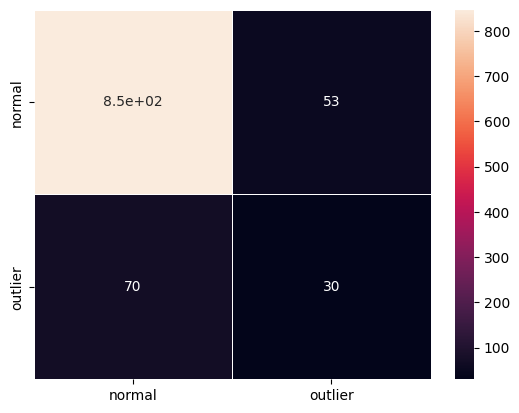
F1 score and confusion matrix:

labels = outlier_batch.target_names
y_pred = od_preds['data']['is_outlier']
f1 = f1_score(y_outlier, y_pred)
print('F1 score: {:.4f}'.format(f1))
cm = confusion_matrix(y_outlier, y_pred)
df_cm = pd.DataFrame(cm, index=labels, columns=labels)
sns.heatmap(df_cm, annot=True, cbar=True, linewidths=.5)
plt.show()

F1 score: 0.3279

Plot instance level outlier scores vs. the outlier threshold:

plot_instance_score(od_preds, y_outlier, labels, od.threshold)

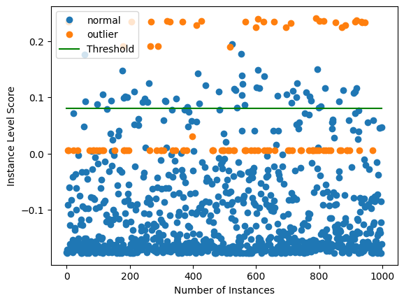
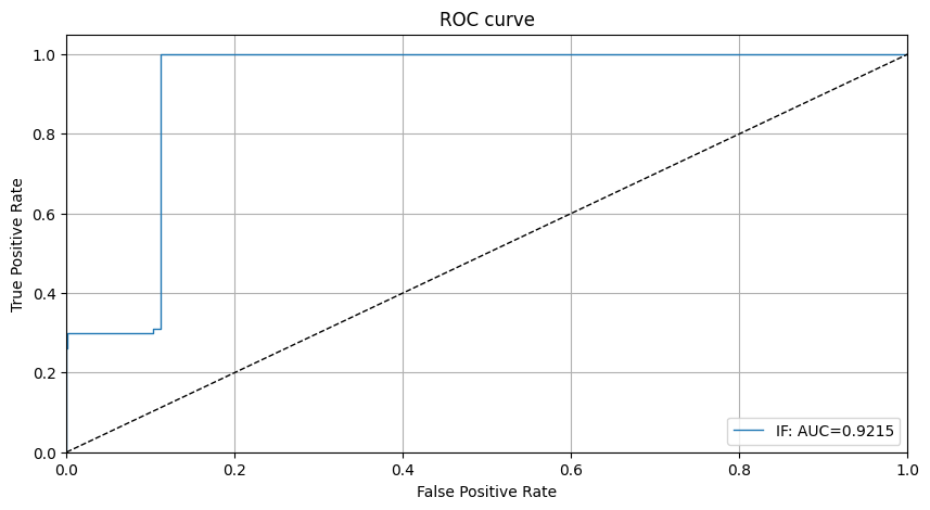
We can see that the isolation forest does not do a good job at detecting 1 type of outliers with an outlier score around 0. This makes inferring a good threshold without explicit knowledge about the outliers hard. Setting the threshold just below 0 would lead to significantly better detector performance for the outliers in the dataset. This is also reflected by the ROC curve:

roc_data = {'IF': {'scores': od_preds['data']['instance_score'], 'labels': y_outlier}}
plot_roc(roc_data)