This page was generated from examples/od_sr_synth.ipynb.

Time series outlier detection with Spectral Residuals on synthetic data

Method

The Spectral Residual outlier detector is based on the paper Time-Series Anomaly Detection Service at Microsoft and is suitable for unsupervised online anomaly detection in univariate time series data. The algorithm first computes the Fourier Transform of the original data. Then it computes the spectral residual of the log amplitude of the transformed signal before applying the Inverse Fourier Transform to map the sequence back from the frequency to the time domain. This sequence is called the saliency map. The anomaly score is then computed as the relative difference between the saliency map values and their moving averages. If this score is above a threshold, the value at a specific timestep is flagged as an outlier. For more details, please check out the paper.

Dataset

We test the outlier detector on a synthetic dataset generated with the TimeSynth package. It allows you to generate a wide range of time series (e.g. pseudo-periodic, autoregressive or Gaussian Process generated signals) and noise types (white or red noise). It can be installed as follows:

!pip install git+https://github.com/TimeSynth/TimeSynth.git

Additionally, this notebook requires the seaborn package for visualization which can be installed via pip:

!pip install seaborn

import matplotlib.pyplot as plt
%matplotlib inline
import numpy as np
import pandas as pd
import seaborn as sns
from sklearn.metrics import accuracy_score, confusion_matrix, f1_score, recall_score
import timesynth as ts

from alibi_detect.od import SpectralResidual
from alibi_detect.utils.perturbation import inject_outlier_ts
from alibi_detect.saving import save_detector, load_detector
from alibi_detect.utils.visualize import plot_instance_score, plot_feature_outlier_ts

Create univariate time series

Define number of sampled points and the type of simulated time series. We use TimeSynth to generate a sinusoidal signal with Gaussian noise.

n_points = 100000

# timestamps
time_sampler = ts.TimeSampler(stop_time=n_points // 4)
time_samples = time_sampler.sample_regular_time(num_points=n_points)

# harmonic time series with Gaussian noise
sinusoid = ts.signals.Sinusoidal(frequency=0.25)
white_noise = ts.noise.GaussianNoise(std=0.1)
ts_harm = ts.TimeSeries(signal_generator=sinusoid, noise_generator=white_noise)
samples, signals, errors = ts_harm.sample(time_samples)
X = samples.reshape(-1, 1).astype(np.float32)
print(X.shape)

(100000, 1)

We can inject noise in the time series via inject_outlier_ts. The noise can be regulated via the percentage of outliers (perc_outlier), the strength of the perturbation (n_std) and the minimum size of the noise perturbation (min_std):

data = inject_outlier_ts(X, perc_outlier=10, perc_window=10, n_std=2., min_std=1.)
X_outlier, y_outlier, labels = data.data, data.target.astype(int), data.target_names
print(X_outlier.shape, y_outlier.shape)

(100000, 1) (100000,)

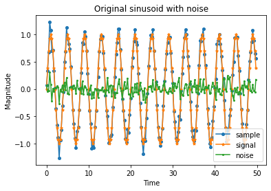
Visualize part of the original and perturbed time series:

n_plot = 200

plt.plot(time_samples[:n_plot], X[:n_plot], marker='o', markersize=4, label='sample')
plt.plot(time_samples[:n_plot], signals[:n_plot], marker='*', markersize=4, label='signal')
plt.plot(time_samples[:n_plot], errors[:n_plot], marker='.', markersize=4, label='noise')
plt.xlabel('Time')
plt.ylabel('Magnitude')
plt.title('Original sinusoid with noise')
plt.legend()
plt.show();

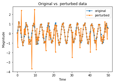
Perturbed data:

plt.plot(time_samples[:n_plot], X[:n_plot], marker='o', markersize=4, label='original')
plt.plot(time_samples[:n_plot], X_outlier[:n_plot], marker='*', markersize=4, label='perturbed')
plt.xlabel('Time')
plt.ylabel('Magnitude')
plt.title('Original vs. perturbed data')
plt.legend()
plt.show();

Define Spectral Residual outlier detector

od = SpectralResidual(
    threshold=None,                  # threshold for outlier score
    window_amp=20,                   # window for the average log amplitude
    window_local=20,                 # window for the average saliency map
    n_est_points=20,                 # nb of estimated points padded to the end of the sequence
    padding_amp_method='reflect',    # padding method to be used prior to each convolution over log amplitude.
    padding_local_method='reflect',  # padding method to be used prior to each convolution over saliency map.
    padding_amp_side='bilateral'     # whether to pad the amplitudes on both sides or only on one side.
)

No threshold level set. Need to infer threshold using `infer_threshold`.

Note that for the local convolution we pad the signal internally only on the left, following the paper’s recommendation.

The warning tells us that we need to set the outlier threshold. This can be done with the infer_threshold method. We need to pass a batch of instances and specify what percentage of those we consider to be normal via threshold_perc. Let’s assume we have some data which we know contains around 10% outliers:

X_threshold = X_outlier[:10000, :]

Let’s infer the threshold:

od.infer_threshold(X_threshold, time_samples[:10000], threshold_perc=90)
print('New threshold: {:.4f}'.format(od.threshold))

New threshold: 1.3632

Let’s save the outlier detector with the updated threshold:

filepath = 'my_path'
save_detector(od, filepath)

Directory my_path does not exist and is now created.

We can load the same detector via load_detector:

od = load_detector(filepath)

Detect outliers

Predict outliers:

od_preds = od.predict(X_outlier, time_samples, return_instance_score=True)

Display results

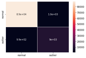
F1 score, accuracy, recall and confusion matrix:

y_pred = od_preds['data']['is_outlier']
f1 = f1_score(y_outlier, y_pred)
acc = accuracy_score(y_outlier, y_pred)
rec = recall_score(y_outlier, y_pred)
print('F1 score: {} -- Accuracy: {} -- Recall: {}'.format(f1, acc, rec))
cm = confusion_matrix(y_outlier, y_pred)
df_cm = pd.DataFrame(cm, index=labels, columns=labels)
sns.heatmap(df_cm, annot=True, cbar=True, linewidths=.5)
plt.show()

F1 score: 0.8983600019939185 -- Accuracy: 0.97961 -- Recall: 0.9011

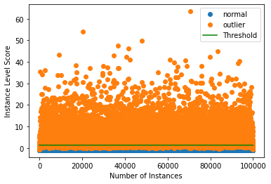
Plot the outlier scores of the time series vs. the outlier threshold. :

plot_instance_score(od_preds, y_outlier, labels, od.threshold)

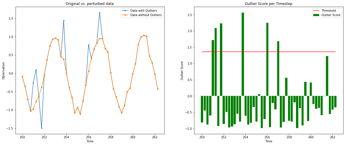
Let’s zoom in on a smaller time scale to have a clear picture:

plot_feature_outlier_ts(od_preds,
                        X_outlier,
                        od.threshold,
                        window=(1000, 1050),
                        t=time_samples,
                        X_orig=X)