This page was generated from examples/integrated_gradients_imagenet.ipynb.
Integrated gradients for a ResNet model trained on Imagenet dataset
In this notebook we apply the integrated gradients method to a pretrained ResNet model trained on the Imagenet data set. Integrated gradients defines an attribution value for each feature (in this case for each pixel and channel in the image) by integrating the model’s gradients with respect to the input along a straight path from a baseline instance \(x^\prime\) to the input instance \(x.\)
A more detailed description of the method can be found here. Integrated gradients was originally proposed in Sundararajan et al., “Axiomatic Attribution for Deep Networks”
Note
To enable support for IntegratedGradients, you may need to run
pip install alibi[tensorflow]
[1]:
import numpy as np
import tensorflow as tf
import matplotlib.pyplot as plt
from alibi.explainers import IntegratedGradients
from tensorflow.keras.applications.resnet_v2 import ResNet50V2
from alibi.datasets import load_cats
from alibi.utils import visualize_image_attr
print('TF version: ', tf.__version__)
print('Eager execution enabled: ', tf.executing_eagerly()) # True
TF version:  2.8.0
Eager execution enabled:  True
Load data
The load_cats function loads a small sample of images of various cat breeds.
[3]:
image_shape = (224, 224, 3)
data, labels = load_cats(target_size=image_shape[:2], return_X_y=True)
print(f'Images shape: {data.shape}')
data = (data / 255).astype('float32')
Images shape: (4, 224, 224, 3)
[4]:
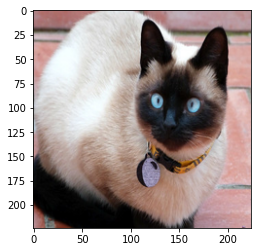
i = 2
plt.imshow(data[i]);
Load model
Load a pretrained tensorflow model with a ResNet architecture trained on the Imagenet dataset.
[5]:
model = ResNet50V2(weights='imagenet')
Calculate integrated gradients
The IntegratedGradients class implements the integrated gradients features attributions method. A description of the method can be found here.
In the first example, the baselines (i.e. the starting points of the path integral) are black images (all pixel values are set to zero). This means that black areas of the image will always have zero attributions. In the second example we consider random uniform noise baselines. The path integral is defined as a straight line from the baseline to the input image. The path is approximated by choosing 50 discrete steps according to the Gauss-Legendre method.
[6]:
n_steps = 50
method = "gausslegendre"
internal_batch_size = 50
ig  = IntegratedGradients(model,
                          n_steps=n_steps,
                          method=method,
                          internal_batch_size=internal_batch_size)
Here we compute attributions for a single image, but batch explanations are supported (leading dimension assumed to be batch).
[7]:
instance = np.expand_dims(data[i], axis=0)
predictions = model(instance).numpy().argmax(axis=1)
explanation = ig.explain(instance,
                         baselines=None,
                         target=predictions)
[8]:
# Metadata from the explanation object
explanation.meta
[8]:
{'name': 'IntegratedGradients',
 'type': ['whitebox'],
 'explanations': ['local'],
 'params': {'method': 'gausslegendre',
  'n_steps': 50,
  'internal_batch_size': 50,
  'layer': 0}}
[9]:
# Data fields from the explanation object
explanation.data.keys()
[9]:
dict_keys(['attributions', 'X', 'forward_kwargs', 'baselines', 'predictions', 'deltas', 'target'])
[10]:
# Get attributions values from the explanation object
attrs = explanation.attributions[0]
Visualize attributions
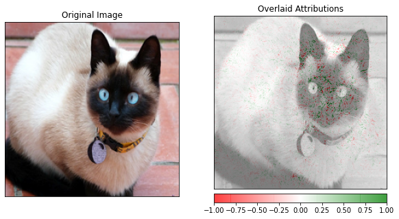
Black image baseline
Sample image from the test set and its attributions. The attributions are shown by overlaying the attributions values for each pixel to the original image. The attribution value for a pixel is obtained by summing up the attributions values for the three color channels. The attributions are scaled in a \([-1, 1]\) range: red pixels represent negative attributions, while green pixels represent positive attributions. The original image is shown in gray scale for clarity.
[11]:
fig, ax = plt.subplots(nrows=1, ncols=2, figsize=(10, 5))
visualize_image_attr(attr=None, original_image=data[i], method='original_image',
                    title='Original Image', plt_fig_axis=(fig, ax[0]), use_pyplot=False);

visualize_image_attr(attr=attrs.squeeze(), original_image=data[i], method='blended_heat_map',
                    sign='all', show_colorbar=True, title='Overlaid Attributions',
                     plt_fig_axis=(fig, ax[1]), use_pyplot=True);

Random baselines
Here we show the attributions obtained choosing random uniform noise as a baseline. It can be noticed that the attributions can be considerably different from the previous example, where the black image is taken as a baseline. An extensive discussion about the impact of the baselines on integrated gradients attributions can be found in P. Sturmfels at al., “Visualizing the Impact of Feature Attribution Baselines”.
[12]:
baselines = np.random.random_sample(instance.shape)
[13]:
explanation = ig.explain(instance,
                         baselines=baselines,
                         target=predictions)
[14]:
attrs = explanation.attributions[0]
Sample image from the test dataset and its attributions. The attributions are shown by overlaying the attributions values for each pixel to the original image. The attribution value for a pixel is obtained by summing up the attributions values for the three color channels. The attributions are scaled in a \([-1, 1]\) range: red pixel represents negative attributions, while green pixels represents positive attributions. The original image is shown in gray scale for clarity.
[15]:
fig, ax = plt.subplots(nrows=1, ncols=2, figsize=(10, 5))
visualize_image_attr(attr=None, original_image=data[i], method='original_image',
                    title='Original Image', plt_fig_axis=(fig, ax[0]), use_pyplot=False);

visualize_image_attr(attr=attrs.squeeze(), original_image=data[i], method='blended_heat_map',
                    sign='all', show_colorbar=True, title='Overlaid Attributions',
                     plt_fig_axis=(fig, ax[1]), use_pyplot=True);