This page was generated from methods/KernelSHAP.ipynb.
Kernel SHAP
Note
To enable SHAP support, you may need to run:
pip install alibi[shap]
Overview
The Kernel SHAP (SHapley Additive exPlanations) algorithm is based on the paper A Unified Approach to Interpreting Model Predictions by Lundberg et al. and builds on the open source shap library from the paper’s first author.
The algorithm provides model-agnostic (black box), human interpretable explanations suitable for regression and classification models applied to tabular data. This method is a member of the additive feature attribution methods class; feature attribution refers to the fact that the change of an outcome to be explained (e.g., a class probability in a classification problem) with respect to a baseline (e.g., average prediction probability for that class in the training set) can be attributed in different proportions to the model input features.
A simple illustration of the explanation process is shown in Figure 1. Here we see depicted a model which takes as an input features such as Age, BMI or Sex and outputs a continuous value. We know that the average value of that output in a dataset of interest is 0.1. Using the Kernel SHAP algorithm, we attribute the 0.3 difference to the input features. Because the sum of the attribute values equals output - base rate, this method is additive. We can see for example
that the Sex feature contributes negatively to this prediction whereas the remainder of the features have a positive contribution. For explaining this particular data point, the Age feature seems to be the most important. See our examples on how to perform explanations with this algorithm and visualise the results using the shap library visualisations here, here and
here.
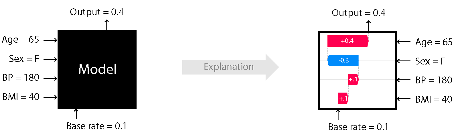 Figure 1: Cartoon illustration of black-box explanation models with Kernel SHAP
Image Credit: Scott Lundberg (see source here)
Usage
In order to compute the shap values , the following hyperparameters can be set when calling the explain method:
nsamples: Determines the number of subsets used for the estimation of the shap values. A default of2*M + 2**11is provided whereMis the number of features. One is encouraged to experiment with the number of samples in order to determine a value that balances explanation accuracy and runtime.l1_reg: can take values0,Falseto disable,autofor automatic regularisation selection,bicoraicto use \(\ell_1\) regularised regression with the Bayes/Akaike information criteria for regularisation parameter selection,num_features(10)to specify the number of feature effects to be returned or a float value that is used as the regularisation coefficient for the \(\ell_1\) penalised regression. The default optionautouses the least angle regression algorithm with the Akaike Information Criterion if a fraction smaller than0.2of the total number of subsets is enumerated.
If the dataset to be explained contains categorical variables, then the following options can be specified unless the categorical variables have been grouped (see example below):
summarise_result: if True, the shap values estimated for dimensions of an encoded categorical variable are summed and a single shap value is returned for the categorical variable. This requires that both arguments below are specified:cat_var_start_idx: a list containing the column indices where categorical variables start. For example if the feature matrix contains a categorical feature starting at index0and one at index10, thencat_var_start_idx=[0, 10].cat_vars_enc_dim: a list containing the dimension of the encoded categorical variables. The number of columns specified in this list is summed for each categorical variable starting with the corresponding index incat_var_start_idx. So ifcat_var_start_idx=[0, 10]andcat_vars_enc_dim=[3, 5], then the columns with indices0, 1and2and10, 11, 12, 13and14will be combined to return one shap value for each categorical variable, as opposed to3and5.
Explaining continuous datasets
Initialisation and fit
The explainer is initialised by specifying:
a predict function.
optionally, setting
link='logit'if the the model to be explained is a classifier that outputs probabilities. This will apply the logit function to convert outputs to margin space.optionally, providing a list of
feature_names
Hence assuming the classifier takes in 4 inputs and returns probabilities of 3 classes, we initialise its explainer as:
from alibi.explainers import KernelShap

predict_fn = lambda x: clf.predict_proba(x)
explainer = KernelShap(predict_fn, link='logit', feature_names=['a','b','c','d'])
To fit our classifier, we simply pass our background or ‘reference’ dataset to the explainer:
explainer.fit(X_reference)
Note that X_reference is expected to have a samples x features layout.
Explanation
To explain an instance X, we simply pass it to the explain method:
explanation = explainer.explain(X)
The returned explanation object has the following fields:
explanation.meta:
{'name': 'KernelShap',
 'type': ['blackbox'],
 'explanations': ['local', 'global'],
 'params': {'groups': None,
            'group_names': None,
            'weights': None,
            'summarise_background': False
           }
}
This field contains metadata such as the explainer name and type as well as the type of explanations this method can generate. In this case, the params attribute shows that none of the fit method optional parameters have been set.
explanation.data:
{'shap_values': [array([ 0.8340445 ,  0.12000589, -0.07984099,  0.61758141]),
                 array([-0.71522546,  0.31749045,  0.3146705 , -0.13365639]),
                 array([-0.12984616, -0.47194649, -0.23036243, -0.52314911])],
 'expected_value': array([0.74456904, 1.05058744, 1.15837362]),
 'link': 'logit',
 'feature_names': ['a', 'b', 'c', 'd'],
 'categorical_names': {},
 'raw': {
     'raw_prediction': array([ 2.23635984,  0.83386654, -0.19693058]),
     'prediction': array([0]),
     'instances': array([ 0.93884707, -0.63216607, -0.4350103 , -0.91969562]),
     'importances': {
         '0': {'ranked_effect': array([0.8340445 , 0.61758141, 0.12000589, 0.07984099]),
               'names': ['a', 'd', 'b', 'c']},
         '1': {'ranked_effect': array([0.71522546, 0.31749045, 0.3146705 , 0.13365639]),
               'names': ['a', 'b', 'c', 'd']},
         '2': {'ranked_effect': array([0.52314911, 0.47194649, 0.23036243, 0.12984616]),
               'names': ['d', 'b', 'c', 'a']},
         'aggregated': {'ranked_effect': array([1.67911611, 1.27438691, 0.90944283, 0.62487392]),
                        'names': ['a', 'd', 'b', 'c']}
         }
     }
}
This field contains:
shap_values: a list of length equal to the number of model outputs, where each entry is an array of dimensionsamples x featuresof shap values. For the example above , only one instance with 4 features has been explained so the shap values for each class are of dimension1 x 4expected_value: an array of the expected value for each model output acrossX_referencelink: which function has been applied to the model output prior to computing theexpected_valueand estimation of theshap_valuesfeature_names: a list with the feature names, if provided. Defaults to a list containing strings of with the formatfeature_{}if no names are passedcategorical_names: a mapping of the categorical variables (represented by indices in theshap_valuescolumns) to the description of the categoryraw: this field contains:raw_prediction: asamples x n_outputsarray of predictions for each instance to be explained. Note that this is calculated by applying the link function specified inlinkto the output ofpred_fnprediction: asamplesarray containing the index of the maximum value in theraw_predictionarrayinstances: asamples x n_featuresarray of instances which have been explainedimportances: a dictionary where each entry is a dictionary containing the sorted average magnitude of the shap value (ranked_effect) along with a list of feature names corresponding to the re-ordered shap values (names). There aren_outputs + 1keys, corresponding ton_outputsand to the aggregated output (obtained by summing all the arrays inshap_values)
Please see our examples on how to visualise these outputs using the shap library visualisations here, here and here.
Explaining heterogeneous (continuous and categorical) datasets
When the dataset contains both continuous and categorical variables, categorical_names, an optional mapping from the encoded categorical features to a description of the category can be passed in addition to the feature_names list. This mapping is currently used for determining what type of summarisation should be applied if X_reference is large and the fit argument summarise_background='auto' or summarise_background=True but in the future it might be used for annotating
visualisations. The definition of the map depends on what method is used to handle the categorical variables.
By grouping categorical data
By grouping categorical data we estimate a single shap value for each categorical variable.
Initialisation and fit
Assume that we have a dataset with features such as Marital Status (first column), Age (2nd column), Income (3rd column) and Education (4th column). The 2nd and 3rd column are continuous variables, whereas the 1st and 4th are categorical ones.
The mapping of categorical variables could be generated from a Pandas dataframe using the utility gen_category_map, imported from alibi.utils. For this example the output could look like:
category_map = {
    0: ["married", "divorced"],
    3: ["high school diploma", "master's degree"],
}
Hence, using the same predict function as before, we initialise the explainer as:
explainer = KernelShap(
    predict_fn,
    link='logit',
    feature_names=["Marital Status", "Age", "Income", "Education"],
    categorical_names=category_map,
)
To group our data, we have to provide the groups list, which contains lists with indices that are grouped together. In our case this would be:
groups = [[0, 1], [2], [3], [4, 5]]
Similarly, the group_names are the same as the feature names
group_names = ["Marital Status", "Age", "Income", "Education"]
Note that, in this case, the keys of the category_map are indices into groups. To fit our explainer we pass one-hot encoded data to the explainer along with the grouping information.
explainer.fit(
    X_reference,
    group_names=group_names,
    groups=groups,
)
Explanation
To perform an explanation, we pass one hot encoded instances X to the explain method:
explanation = explainer.explain(X)
The explanation returned will contain the grouping information in its meta attribute
{'name': 'KernelShap',
 'type': ['blackbox'],
 'explanations': ['local', 'global'],
 'params': {'groups': [[0, 1], [2], [3], [4, 5]],
            'group_names': ["Marital Status", "Age", "Income", "Education"] ,
            'weights': None,
            'summarise_background': False
           }
}
whereas inspecting the data attribute shows that one shap value is estimated for each of the four groups:
{'shap_values': [array([ 0.8340445 ,  0.12000589, -0.07984099,  0.61758141]),
                 array([-0.71522546,  0.31749045,  0.3146705 , -0.13365639]),
                 array([-0.12984616, -0.47194649, -0.23036243, -0.52314911])],
 'expected_value': array([0.74456904, 1.05058744, 1.15837362]),
 'link': 'logit',
 'feature_names': ["Marital Status", "Age", "Income", "Education"],
 'categorical_names': {},
 'raw': {
     'raw_prediction': array([ 2.23635984,  0.83386654, -0.19693058]),
     'prediction': array([0]),
     'instances': array([ 0.93884707, -0.63216607, -0.4350103 , -0.91969562]),
     'importances': {
         '0': {'ranked_effect': array([0.8340445 , 0.61758141, 0.12000589, 0.07984099]),
               'names': ['a', 'd', 'b', 'c']},
         '1': {'ranked_effect': array([0.71522546, 0.31749045, 0.3146705 , 0.13365639]),
               'names': ['a', 'b', 'c', 'd']},
         '2': {'ranked_effect': array([0.52314911, 0.47194649, 0.23036243, 0.12984616]),
               'names': ['d', 'b', 'c', 'a']},
         'aggregated': {'ranked_effect': array([1.67911611, 1.27438691, 0.90944283, 0.62487392]),
                        'names': ['a', 'd', 'b', 'c']}
         }
     }
}
By summing output
An alternative to grouping, with a higher runtime cost, is to estimate one shap value for each dimension of the one-hot encoded data and sum the shap values of the encoded dimensions to obtain only one shap value per categorical variable.
Initialisation and fit
The initialisation step is as before:
explainer = KernelShap(
    predict_fn,
    link='logit',
    feature_names=["Marital Status", "Age", "Income", "Education"],
    categorical_names=category_map,
)
However, note that the keys of the category_map have to correspond to the locations of the categorical variables after the effects for the encoded dimensions have been summed up (see details below).
The fit step requires one hot encoded data and simply takes the reference dataset:
explainer.fit(X_reference)
Explanation
To obtain a single shap value per categorical result, we have to specify the following arguments to the explain method:
summarise_result: indicates that some shap values will be summedcat_vars_start_idx: the column indices where the first encoded dimension is for each categorical variablecat_vars_enc_dim: the length of the encoding dimensions for each categorical variable
explanation = explainer.explain(
    X,
    summarise_result=True,
    cat_vars_start_idx=[0, 4],
    cat_vars_enc_dim=[2, 2],
)
In our case Marital Status starts at column 0 and occupies 2 columns, Age and Income occupy columns 2 and 3 and Education occupies columns 4 and 5.
By combining preprocessor and predictor
Finally, an alternative is to combine the preprocessor and the predictor together in the same object, and fit the explainer on data before preprocessing.
Initialisation and fit
To do so, we first redefine our predict function as
predict_fn = lambda x: clf.predict(preprocessor.transform(x))
The explainer can be initialised as:
explainer = KernelShap(
    predict_fn,
    link='logit',
    feature_names=["Marital Status", "Age", "Income", "Education"],
    categorical_names=category_map,
)
Then, the explainer should be fitted on unprocessed data:
explainer.fit(X_referennce_unprocessed)
Explanation
We can explain unprocessed records simply by calling explain:
explanation = explainer.explain(X_unprocessed)
Running batches of explanations in parallel
Increases in the size of the background dataset, the number of samples used to estimate the shap values or simply explaining a large number of instances dramatically increase the cost of running Kernel SHAP.
To explain batches of instances in parallel, first run pip install alibi[ray] to install required dependencies and then simply initialise KernelShap specifying the number of physical cores available as follows:
distrib_kernel_shap = KernelShap(predict_fn, distributed_opts={'n_cpus': 10}
To explain, simply call the explain as before - no other changes are required.
Warning
Windows support for the ray Python library is still experimental. Using KernelShap in parallel is not currently supported on Windows platforms.
Miscellaneous
Runtime considerations
For a given instance, the runtime of the algorithm depends on:
the size of the reference dataset
the dimensionality of the data
the number of samples used to estimate the shap values
Adjusting the size of the reference dataset
The algorithm automatically warns the user if a background dataset size of more than 300 samples is passed. If the runtime of an explanation with the original dataset is too large, then the algorithm can automatically subsample the background dataset during the fit step. This can be achieve by specifying the fit step as
explainer.fit(
    X_reference,
    summarise_background=True,
    n_background_samples=150,
)
or
explainer.fit(
    X_reference,
    summarise_background='auto'
)
The auto option will select 300 examples, whereas using the boolean argument allows the user to directly control the size of the reference set. If categorical variables or grouping options are specified, the algorithm uses subsampling of the data. Otherwise, a kmeans clustering algorithm is used to select the background dataset and the samples are weighted according to the frequency of occurrence of the cluster they are assigned to, which is reflected in the expected_value attribute
of the explainer.
As described above, the explanations are performed with respect to the expected (or weighted-average) output over this dataset so the shap values will be affected by the dataset selection. We recommend experimenting with various ways to choose the background dataset before deploying explanations.
The dimensionality of the data and the number of samples used in shap value estimation
The dimensionality of the data has a slight impact on the runtime, since by default the number of samples used for estimation is 2*n_features + 2**11. In our experiments, we found that either grouping the data or fitting the explainer on unprocessed data resulted in run time savings (but did not run rigorous comparison experiments). If grouping/fitting on unprocessed data alone does not give enough runtime savings, the background dataset could be adjusted. Additionally (or alternatively),
the number of samples could be reduced as follows:
explanation = explainer.explain(X, nsamples=500)
We recommend experimenting with this setting to understand the variance in the shap values before deploying such configurations.
Imbalanced datasets
In some situations, the reference datasets might be imbalanced so one might wish to perform an explanation of the model behaviour around \(x\) with respect to \(\sum_{i} w_i f(y_i)\) as opposed to \(\mathbb{E}_{\mathcal{D}}[f(y)]\). This can be achieved by passing a list or an 1-D numpy array containing a weight for each data point in X_reference as the weights argument of the fit method.
Theoretical overview
Consider a model \(f\) that takes as an input \(M\) features. Assume that we want to explain the output of the model \(f\) when applied to an input \(x\). Since the model output scale does not have an origin (it is an affine space), one can only explain the difference of the observed model output with respect to a chosen origin point. This point can be taken to be the function output value for an arbitrary record or the average output over a set of records, \(\mathcal{D}\). Assuming the latter case, for the explanation to be accurate, one requires
where \(\mathcal{D}\) is also known as a background dataset and \(\phi_i\) is the portion of the change attributed to the \(i\)th feature. This portion is sometimes referred to as feature importance, effect or simply shap value.
One can conceptually imagine the estimation process for the shap value of the \(i^{th}\) feature \(x_i\) as consisting of the following steps:
enumerate all subsets \(S\) of the set \(F = \{1, ..., M\} \setminus \{i\}\)
for each \(S \subseteq F \setminus \{i\}\), compute the contribution of feature \(i\) as \(C(i|S) = f(S \cup \{i\}) - f(S)\)
compute the shap value according to
\[\phi_i := \frac{1}{M} \sum \limits_{{S \subseteq F \setminus \{i\}}} \frac{1}{\binom{M - 1}{|S|}} C(i|S).\]
The semantics of \(f(S)\) in the above is to compute \(f\) by treating \(\bar{S}\) as missing inputs. Thus, we can imagine the process of computing the SHAP explanation as starting with \(S\) that does not contain our feature, adding feature \(i\) and then observing the difference in the function value. For a nonlinear function the value obtained will depend on which features are already in \(S\), so we average the contribution over all possible ways to choose a subset of size \(|S|\) and over all subset sizes. The issue with this method is that:
the summation contains \(2^M\) terms, so the algorithm complexity is \(O(M2^M)\)
since most models cannot accept an arbitrary pattern of missing inputs at inference time, calculating \(f(S)\) would involve model retraining the model an exponential number of times
To overcome this issue, the following approximations are made:
the missing features are simulated by replacing them with values from the background dataset
the feature attributions are estimated instead by solving
where
is the Shapley kernel (Figure 2).
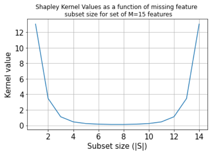
Figure 2: Shapley kernel
Note that the optimisation objective implies above an exponential number of terms. In practice, one considers a finite number of samples n, selecting n subsets \(S_1, ..., S_n\) according to the probability distribution induced by the kernel weights. We can see that the kernel favours either small or large subset sizes, since most of the information about the effect of a particular feature for an outcome change can be obtained by excluding that feature or excluding all the features
except for it from the input set.
Therefore, Kernel SHAP returns an approximation of the true Shapley values, whose variability depends on factors such as the size of the structure of the background dataset used to estimate the feature attributions and the number of subsets of missing features sampled. Whenever possible, algorithms specialised for specific model structures (e.g., Tree SHAP, Linear SHAP, integrated gradients) should be used since they are faster and more accurate.
Comparison to other methods
Like LIME, this method provides local explanations, in the sense that the attributions are estimated to explain the change from a baseline for a given data point, \(x\). LIME computes the feature attributions by optimising the following objective in order to obtain a locally accurate explanation model (i.e., one that approximates the model to explained well around an instance \(x\)):
Here \(f\) is the model to be explained, \(g\) is the explanation model (assumed linear), \(\pi\) is a local kernel around instance \(x\) (usually cosine or \(\ell_2\) kernel) and \(\Omega(g)\) penalises explanation model complexity. The choices for \(L, \pi\) and \(\Omega\) in LIME are heuristic, which can lead to unintuitive behaviour (see Section 5 of Lundberg et al. for a study). Instead, by computing the shap values according to the weighted regression in the previous section, the feature attributions estimated by Kernel SHAP have desirable properties such as local accuracy , consistency and missingness, detailed in Section 3 of Lundberg et al..
Although, in general, local explanations are limited in that it is not clear to what a given explanation applies around and instance \(x\) (see anchors algorithm overview here for a discussion), insights into global model behaviour can be drawn by aggregating the results from local explanations (see the work of Lundberg et al. here). In the future, a distributed version of the Kernel SHAP algorithm will be available in order to reduce the runtime requirements necessary for explaining large datasets.
Examples
Continuous Data
Mixed Data
Handling categorical variables with Kernel SHAP: an income prediction application
Handlling categorical variables with Kernel SHAP: fitting explainers on data before pre-processing
Distributed Kernel SHAP: paralelizing explanations on multiple cores