This page was generated from methods/PartialDependence.ipynb.

[source]

Partial Dependence

Overview

The partial dependence (PD) plot proposed by J.H. Friedman (2001)[1], is a method to visualize the marginal effect that one or two features have on the predicted outcome of a machine learning model. By inspecting the PD plots, one can understand whether the relation between a feature/pair of features is, for example, a simple linear or quadratic relation, whether it presents a monotonically increasing or decreasing trend, or reveal a more complex response.

The following figure displays two one-way PD plots for two features and a one two-way PD for the same features. The prediction model is random forest regression trained on the Bike rental[2] dataset (see worked example).

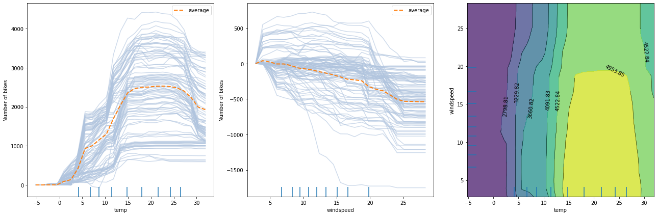
From the left plot, we can observe that the average model prediction increases with the temperature till it reaches approximately \(17^\circ C\). Then it flattens at a high number until the weather becomes too hot (i.e. approx. \(27^\circ C\)), after which it starts dropping again. A similar analysis can be conducted by inspecting the middle figure for wind speed. As the wind speed increases, fewer and fewer people are riding the bike. Finally, by looking at the right plot, we can visualize how the two features interact. In a few words, the plot suggests that for relatively warm weather, the number of rentals increases as long as the wind is not too rough. For a more detailed analysis, please check the worked example.

For pros & cons of PD plots, see the Partial Dependence section from the Introduction materials.

Usage

To initialize the explainer with any black-box model one can directly pass the prediction function and optionally a list of feature names, a list of target names, and a dictionary of categorical names for interpretation and specification of the categorical features:

from alibi.explainers import PartialDependence
pd = PartialDependence(predictor=prediction_fn,
                       feature_names=feature_names,
                       categorical_names=categorical_names,
                       target_names=target_names)

In addition, similar to the sklearn implementation, alibi supports a faster PD computation for some tree-based sklearn models through the TreePartialDependence explainer. The initialization is similar to the one above, with the difference that the predictor argument will be set to the tree predictor object instead of the prediction function.

from alibi.explainer import TreePartialDependence
tree_pd = TreePartialDependence(predictor=tree_predictor,
                                feature_names=feature_names,
                                categorical_names=categorical_names,
                                target_names=target_name)

Following the initialization, we can produce an explanation given a dataset \(X\):

exp = pd.explain(X=X,
                 features=features,
                 kind='average')

Multiple arguments can be provided to the explain method:

• X - A N x F tabular dataset used to calculate partial dependence curves. This is typically the training dataset or a representative sample.

• features - An optional list of features or pairs of features for which to calculate the partial dependence. If not provided, the partial dependence will be computed for every single features in the dataset. Some example for features would be: [0, 2], [0, 2, (0, 2)], [(0, 2)], where 0 and 2 correspond to column 0 and 2 in X, respectively.

• kind - If set to 'average', then only the partial dependence (PD) averaged across all samples from the dataset is returned. If set to individual, then only the individual conditional expectation (ICE) is returned for each individual from the dataset. Otherwise, if set to 'both', then both the PD and the ICE are returned.

• percentiles - Lower and upper percentiles used to limit the feature values to potentially remove outliers from low-density regions. Note that for features with not many data points with large/low values, the PD estimates are less reliable in those extreme regions. The values must be in [0, 1]. Only used with grid_resolution.

• grid_resolution - Number of equidistant points to split the range of each target feature. Only applies if the number of unique values of a target feature in the reference dataset X is greater than the grid_resolution value. For example, consider a case where a feature can take the following values: [0.1, 0.3, 0.35, 0.351, 0.4, 0.41, 0.44, ..., 0.5, 0.54, 0.56, 0.6, 0.65, 0.7, 0.9], and we are not interested in evaluating the marginal effect at every single point as it can become computationally costly (assume hundreds/thousands of points) without providing any additional information for nearby points (e.g., 0.35 and 351). By setting grid_resolution=5, the marginal effect is computed for the values [0.1, 0.3, 0.5, 0.7, 0.9] instead, which is less computationally demanding and can provide similar insights regarding the model’s behaviour. Note that the extreme values of the grid can be controlled using the percentiles argument.

• grid_points - Custom grid points. Must be a dict where the keys are the target features indices and the values are monotonically increasing numpy arrays defining the grid points for numerical feature, and a subset of categorical feature values for a categorical feature. If the grid_points are not specified, then the grid will be constructed based on the unique target feature values available in the reference dataset X, or based on the grid_resolution and percentiles (check grid_resolution to see when it applies). For categorical features, the corresponding value in the grid_points can be specified either as numpy array of strings or numpy array of integers corresponding the label encodings. Note that the label encoding must match the ordering of the values provided in the categorical_names.

Note that for the tree explainer, we no longer have the option to select the kind argument since the TreePartialDependece can only compute the PD and not the ICE. In this case, the explain call should look like this:

tree_exp = tree_pd.explain(X=X,
                           features=features)

The rest of the arguments are still available.

The result exp/tree_exp is an Explanation object which contains the following data-related attributes:

• feature_values - A list of arrays or list of arrays containing the evaluation points for each explained feature passed in the features argument (see explain method).

• feature_names - A list of strings or tuples of string containing the names associated with the explained features elements from feature_values.

• feature_deciles - a list of arrays (one for each numerical features) of the explained feature deciles.

• pd_values - a list of arrays of PD values (one for each feature/pair of features). Each array has a shape of T x (V1 x V2 x ...), where T is the number of target outputs, and Vi is the number of evaluation points for the corresponding feature fi.

• ice_values - a list of arrays of ICE values (one for each feature/pair of feature). Each array has a shape of T x N x (V1 x V2 x ...), where T is the number of target outputs, N is the number of instances in the reference dataset, and Vi is the number of evaluation points for the corresponding feature fi. For TreePartialDependence the value of this attribute is None.

Plotting the pd_values and ice_values against exp_feature_values recovers the PD and the ICE plots, respectively. For convenience we included a plotting function plot_pd which automatically produces PD and ICE plots using matplotlib.

from alibi.explainers import plot_pd
plot_pd(exp)

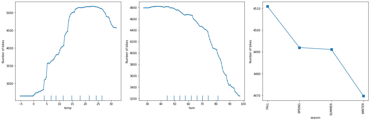
The following figure displays the one way PD plots for a random forest regression trained on the Bike rental[2] dataset (see worked example).

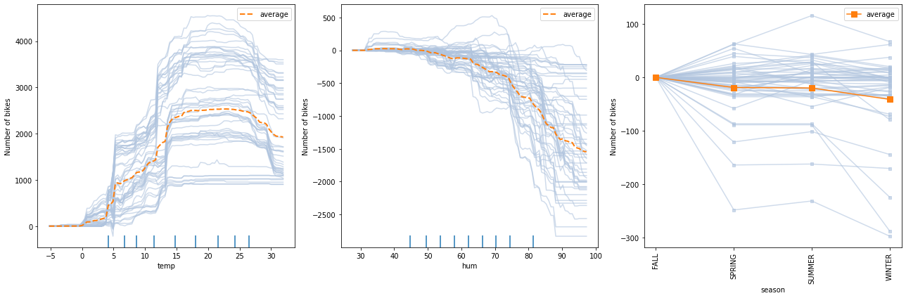
The following figure displays the ICE plots for a random forest regression trained on the Bike rental[2] dataset (see worked example).

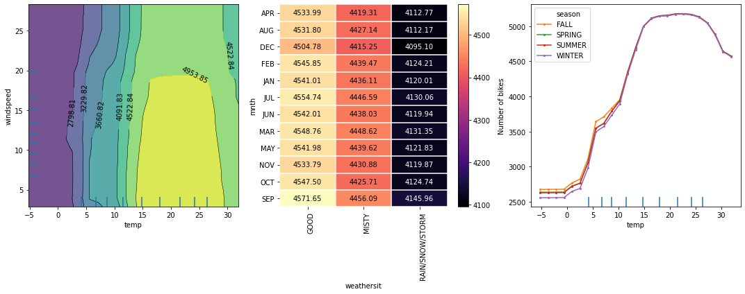
The following figure displays the two way PD plots for a random forest regression trained on the Bike rental[2] dataset (see worked example).

Theoretical exposition

Before diving into the mathematical formulation of the PD, we first introduce some notation. Consider \(\mathcal{F}\) to be the set of all features, \(S\) be a set of features of interest (i.e. \(S \subseteq \mathcal{F}\)) that we want to compute the marginal effect for, and \(C\) be their complement (i.e. \(C = \mathcal{F} \setminus S\)). It is important to note that the subset \(S\) is not only restricted to one or two features as mentioned in the previous paragraph but can be any subset of the set \(\mathcal{F}\). In practice, though, due to visualization reasons, we will not analyze more than two features at a time.

Given a black-box model, \(f\), we are ready to define the partial dependence for a set of features \(S\) as:

\[f_{S}(x_S) = \mathbb{E}_{X_C} [f(x_S, X_C)] = \int f(x_S, X_C) d\mathbb{P}(X_C),\]

where we denoted random variables by capital letters (e.g., \(X_C\)), realizations by lowercase letters (e.g. \(x_S\)), and \(\mathbb{P}(X_C)\) the probability distribution/measure over the features set C.

In practice, to approximate the integral above, we compute the average over a reference dataset. Formally, let us consider a reference dataset \(\mathcal{X} = \{x^{(1)}, x^{(2)}, ..., x^{(n)}\}\). The PD for the set \(S\) can be approximated as:

\[f_{S}(x_S) = \frac{1}{n} \sum_{i=1}^{n}f(x_S, x_{C}^{(i)}).\]

In simple words, to compute the marginal effect of the feature values \(x_S\), we query the model on synthetic instances created from the concatenation of \(x_S\) with the feature values \(x_C^{(i)}\) from the reference dataset and average the model responses. Already from the computation, we can identify a major limitation of the method. The PD computation assumes feature independence (i.e., features are not correlated) which is a strong and quite restrictive assumption and usually does not hold in practice. A classic example of positively correlated features is height and weight. If \(S = \{\text{height}\}\) and \(C=\{\text{weight}\}\), the independence assumption will create an unrealistic synthetic instance, by combining values of height and weight that are not correlated (e.g. \(\text{height} = 1.85\text{m}\) - height of an adult - and \(\text{weight} = 30 \text{kg}\) - weight of a child). This limitation can be addressed by the Accumulated Local Effects[3] (ALE) method.

Although the ALE can handle correlated features, the PD still has some advantages beyond their simple and intuitive definition. The PD can directly be extended to categorical features. For each category of a feature, one can compute the PD by setting all data instance to have the same category and following the same averaging strategy over the reference dataset (i.e., replace features \(C\) with feature values from the reference, compute the response, and average all the responses). Note that ALE requires by definition the feature values to be ordinal, which might not be the case for all categorical features. Depending on the context, there exist some methods that allow the ALE to be extended to categorical features for which we recommend the ALE chapter from the Interpretable machine learning[4] book, as further reading.

We illustrate PD for the simple case of interpreting a linear regression model and demonstrate that it correctly results in showing a linear relationship between the features and the response. To formally prove the linear relationship, consider the following linear regression model:

\[f(x) = \beta_0 + \beta_1 x_1 + ... \beta_{|\mathcal{F}|} x_{|\mathcal{F}|}.\]

Without loss of generality, we can assume the features of interest come first in the equation above and the rest of the features at the end. We can rewrite the above equation as follows:

\[f(x) = \beta_0 + \beta_1 x_{S_1} + ... + \beta_{|S|} x_{S_{|S|}} + \beta_{|S| + 1} x_{C_{1}} + ... + \beta_{|S| + |C|} x_{C_{|C|}},\]

where \(S_{i}\) and \(C_{i}\) represent features in \(S\) and \(C\), respectively.

Following the definition of PD, we obtain:

\begin{align} f_S(x_{S}) &= \mathbb{E}_{X_C}[f(x_S, X_C)] \\ & = \mathbb{E}_{X_C}[\beta_0 + \beta_1 x_{S_1} + ... + \beta_{\lvert S\rvert} x_{S_{\lvert S\rvert}} + \beta_{\lvert S\rvert + 1} x_{C_{1}} + ... + \beta_{\lvert S\rvert + \lvert C\rvert} x_{C_{\lvert C\rvert}}] \\ & = \beta_0 + \beta_1 x_{S_1} + ... + \beta_{\lvert S\rvert} x_{S_{\lvert S\rvert}} + \mathbb{E}_{X_C}[x_{C_{1}} + ... + \beta_{\lvert S\rvert + \lvert C\rvert} x_{C_{\lvert C\rvert}}] \\ & = \beta_0 + \beta_1 x_{S_1} + ... + \beta_{\lvert S\rvert} x_{S_{\lvert S\rvert}} + K_C \\ & = (\beta_0 + K_C) + \beta_1 x_{S_1} + ... + \beta_{\lvert S\rvert} x_{S_{\lvert S\rvert}}. \end{align}

The following figure displays the PD plots for a linear regression model trained on the for Bike rentals[2] dataset:

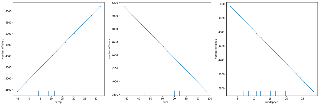
As expected, we observe a linear relation between the feature value and the marginal effect.

Examples

PD, ICE regression example (Bike rental)

References

[1] Friedman, Jerome H. “Greedy function approximation: a gradient boosting machine.” Annals of statistics (2001): 1189-1232.

[2] Fanaee-T, Hadi, and Gama, Joao, ‘Event labeling combining ensemble detectors and background knowledge’, Progress in Artificial Intelligence (2013): pp. 1-15, Springer Berlin Heidelberg.

[3] Apley, Daniel W., and Jingyu Zhu. “Visualizing the effects of predictor variables in black box supervised learning models.” Journal of the Royal Statistical Society: Series B (Statistical Methodology) 82.4 (2020): 1059-1086.

[4] Molnar, Christoph. Interpretable machine learning. Lulu. com, 2020.