This page was generated from methods/PermutationImportance.ipynb.

Permutation Importance

Overview

The permutation importance, initially proposed by Breiman (2001)[1], and further refined by Fisher et al. (2019)[2] is a method to compute the global importance of a feature for a tabular dataset. The computation of the feature importance is based on how much the model performance degrades when the feature values within a feature column are permuted. By inspecting the attribution received by each feature, a practitioner can understand which are the most important features that the model relies on to compute its predictions.

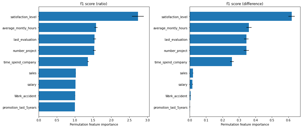
Permutation Importance using F1 score, Who's Going to Leave Next?.

Figure 1. Permutation Importance using \(F_1\) score on “Who’s Going to Leave Next?” dataset. Left figure displays the importance as the ratio between the original score and the permuted score. Right figure displays the importance as the difference between the original score and the permuted score.

Figure 1 displays the importance of each feature according to the \(F_1\) score function reported as the ratio between the original score and the permuted score (left plot), and as the difference between the original score and the permuted score (right plot). We can observe that the most important feature that the model relies on is the satisfaction level. Following that, we have three features that have approximately the same importance, namely the average_montly_hours, last_evaluation and number_project. Finally, in our top 5 hierarchy we have time_spend_company. Features like sales, salary, Work_accident and promotion_last_5years receive an importance close to 1 in the left plot and an importance close to 0 in the right plot which are an indication that the features are not important to the model. For a more detailed analysis, please check the worked example.

For pros & cons, see the Permutation Importance section from the Introduction materials.

Usage

To initialize the explainer with any black-box model, one can directly pass the prediction function, the metrics consisting of the loss functions or the score functions, and optionally a list of feature names:

from alibi.explainers import PermutationImportance

pfi = PermutationImportance(predictor=predict_fn,
                            loss_fns=loss_fns,
                            score_fns=score_fns,
                            feature_names=feature_names)

Note

Remember that the PermutationImportance explainer measures the importance of a feature f as the degradation of the model when the feature values of f are permuted. The degradation of the model can thus be quantified as either the increase in the loss function or the decrease in the score function. Although one can transform a loss function into a score function an vice-versa (i.e., simply negate the value and optionally add an offset), the equivalent representation might not be always be natural to interpret (e.g., transforming mean squared error loss into the equivalent score given by the negative mean squared error). Thus, the alibi API allows the user to provide the suitable metric either as a loss or a score function.

The metric (loss or score) functions can be initialized through strings, a callable or dictionaries. For example, for a classification problem, the initialization of the score functions through strings can be done either score_fns = ['accuracy', 'f1'] or directly score_fns='f1' when a single score function is used. Similarly, when a singe score function is used the initialization through a callable can be done as score_fns = accuracy_score, where accuracy_score is the reference to the function. Finally, the initialization through a dictionary would look like score_fns={'name_score_1': function_score_1, 'name_score_2': function_score_2}. For all the previous cases, the initialization is analogous for the loss functions.

Note that the initialization through a callable or a dictionary allows the flexibility to provide custom metric functions. The signature of a metric function must be as follows:

def metric_fn(y_true: np.ndarray,
              y_pred: np.ndarray,
              sample_weight: Optional[np.ndarray] = None) -> float:
    pass

or

def metric_fn(y_true: np.ndarray,
              y_score: np.ndarray,
              sample_weight: Optional[np.ndarray] = None) -> float:
    pass

where y_true is the array of ground-truth values, y_pred | y_score is the output of the predictor used in the initialization of the explainer, and sample_weight is an optional array containing the weights for the given data instances.

Besides designing custom metrics, the signature above makes it possible to use the sklearn metrics provided here. Also, the list of all supported string metrics can be found here.

Following the initialization, we can produce an explanation given the test dataset \((X_\text{test}, y_\text{test})\):

exp = pfi.explain(X=X_test, y=y_test)

Multiple arguments can be provided to the explain method:

X - A N x F input feature dataset used to calculate the permutation feature importance. This is typically the test dataset.
y - Ground-truth labels array of size N (i.e. (N, )) corresponding the input feature X.
features - An optional list of features or tuples of features for which to compute the permutation feature importance. If not provided, the permutation feature importance will be computed for every single features in the dataset. Some example of features would be: [0, 2], [0, 2, (0, 2)], [(0, 2)], where 0 and 2 correspond to column 0 and 2 in X, respectively.
method - The method to be used to compute the feature importance. If set to 'exact', a “switch” operation is performed across all observed pairs, by excluding pairings that are actually observed in the original dataset. This operation is quadratic in the number of samples (N x (N - 1) samples) and thus can be computationally intensive. If set to 'estimate', the dataset will be divided in half. The values of the first half containing the ground-truth labels the rest of the features (i.e. features that are left intact) is matched with the values of the second half of the permuted features, and the other way around. This method is computationally lighter and provides estimate error bars given by the standard deviation. Note that for some specific loss and score functions, the estimate does not converge to the exact metric value.
kind - Whether to report the importance as the loss/score ratio or the loss/score difference. Available values are: 'ratio' | 'difference'.
n_repeats - Number of times to permute the feature values. Considered only when method='estimate'.
sample_weight - Optional weight for each sample instance.

Note

As mentioned in the parameter description, depending on the loss or score functions used to measure the model performance, the feature importance values when using method='estimate' might not converge to the feature importance values when method='exact', regardless of the number of times the feature values are permuted specified via n_repeats.

The result exp is an Explanation object which contains the following data-related attributes:

feature_names - A list of strings or tuples of strings containing the names associated with the explained features.
metric_names - A list of strings containing the names of the metrics used to compute the feature importance.
feature_importance - A list of lists of float when method='exact' and list of lists of dictionary when method='estimate' containing the feature importance for each metric and each explained feature. When method='estimate', the dictionary returned for each metric and each feature contains the importance mean, the importance standard deviation and the samples used to compute those statistics.

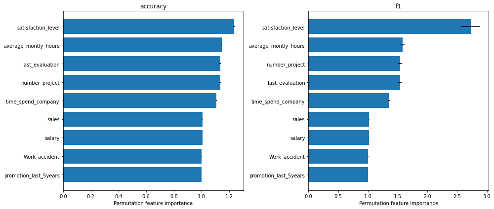
For convenience, we included a plotting function plot_permutation_importance which produces a bar plot with the feature importance values for each metric using matplotlib.

from alibi.explainers import plot_permutation_importance
plot_permutation_importance(exp)

The following figure displays the feature importance for the accuracy and \(F_1\) score for a random forest classifier trained on the “Who’s Going to Leave Next?” dataset (see worked example).

Permutation importance for accuracy and F1 score.

Theoretical exposition

Breiman (2001)[1] initially proposed the permutation feature importance for a random forest classifier as a method to compute the global importance of a feature as seen by the model. More precisely, consider a dataset with \(M\) input features and a random forest classifier. After each tree is created, the values of the \(m\)-th feature in the out-of-bag (OOB) split are randomly permuted and the newly generated data is fed to the current tree to obtain a new prediction. The result for each newly generated data instance from OOB is saved. The process is then repeated for all features \(m = 1, 2, ..., M\). After the procedure is completed for every tree, the noised responses are compared with the true label to give the misclassification rate. The importance of each feature is given by the percent increase in the misclassification rate as compared with the OOB rate when all the features are left intact.

Note

The intuition behind the procedure described above is that an increase in the misclassification rate is an indication that a feature is important for the given model.

Although the method was initially proposed for a random forest classifier, it can be easily generalized to any model and prediction task (e.g., classification or regression). Fisher et al. (2019)[2] proposed a model agnostic version of the permutation feature importance called model reliance which is the one implemented in alibi.

Notation

Before diving into the mathematical formulation of the model reliance, we first introduce some notation. Let \(Z=(Y, X_1, X_2) \in \mathcal{Z}\) be an iid random variable with outcome \(Y \in \mathcal{Y}\) and covariates (features) \(X = (X_1, X_2) \in \mathcal{X}\), where the covariates subsets \(X_1 \in \mathcal{X}_1\) and \(X_2 \in \mathcal{X}_2\) may be each multivariate. The goal is to measure how much the model prediction relies on \(X_1\) to predict \(Y\).

For a given prediction model \(f\), Fisher et al. (2019)[2] introduced the model reliance to be the percent increase in \(f\)’s expected loss when noise is added to \(X_1\). Informally this can be written as:

\[MR(f) = \frac{\text{Expected loss of } f \text{ under noise}}{\text{Expected loss of } f \text{ without noise}}\]

Note that there are certain properties that the noise must satisfy:

must render \(X_1\) completely uninformative of the outcome \(Y\).
must not alter the marginal distribution of \(X_1\).

Definition

Given the notation above, we can introduce formally the model reliance.

Let \(Z^{(a)} = (Y^{(a)}, X_1^{(a)}, X_2^{(b)})\) and \(Z^{(b)} = (Y^{(b)}, X_1^{(b)}, X_2^{(b)})\) be independent random variables, each following the same distribution as \(Z = (Y, X_1, X_2)\). The expected loss of the model \(f\) across pairs of observations \((Z^{(a)}, Z^{(b)})\) in which the values \(X_1^{(a)}\) and \(X_{1}^{(b)}\) have been switched is defined as:

\[e_{\text{switch}}(f) = \mathbb{E}[L\{f, (Y^{(b)}, X_1^{(a)}, X_2^{(b)})\}]\]

Note that the definition above uses the pair \((Y^{(b)}, X_2^{(b)})\) from \(Z^{(b)}\), but the variable \(X_1^{(a)}\) from \(Z^{(a)}\), hence the name switched. It is important to understand that the values \((Y^{(b)}, X_1^{(a)}, X_2^{(b)})\) do not relate to each other and thus we brake the correlation between \(X_1\) with the remaining features \(X_2\) and with the output \(Y\). An alternative interpretation of \(e_{\text{switch}}(f)\) is the expected loss of \(f\) when noise is added to \(X_1\) in such a way that \(X_1\) becomes completely uninformative of \(Y\), but the marginal of \(X_1\) is unchanged.

The reference quantity to compare \(e_{\text{switch}}(f)\) against is the standard expected loss when the features are left intact (i.e., none of the feature values were switched). Formally it can be written as:

\[e_{\text{orig}}(f) = \mathbb{E}[L\{f, (Y, X_1, X_2)\}]\]

Given the two quantities above, we can formally define \(MR(f)\) as their ratio:

\[MR(f) = \frac{e_{\text{switch}}(f)}{e_{\text{orig}}(f)}\]

There are three possible cases to be analyzed:

\(MR(f) > 1\) indicates that the model \(f\) relies on the feature \(X_1\). For example, a \(MR(f) = 2\) means that the error loss has doubled when \(X_1\) was permuted.
\(MR(f) = 1\) indicates that the model \(f\) does not rely on the feature \(X_1\). This means that the error has not changed when \(X_1\) was permuted.
\(MR(f) < 1\) is an interesting case. Surprisingly, there exist models \(f\) such that their reliance is less than one. For example, this can happen if the model \(f\) treats \(X_1\) and \(Y\) as positively correlated when in fact they are negatively correlated. In many cases, a \(MR(f) < 1\) implies the existence of a better performant model \(f^\prime\) satisfying \(MR(f^\prime) = 1\) and \(e_{\text{orig}}(f^\prime) < e_{\text{orig}}(f)\). This is equivalent to saying that the model \(f\) is typically suboptimal.

An alternative definition of the model reliance which uses the difference instead of the ratio is given by:

\[MR_{\text{difference}}(f) = e_{\text{switch}}(f) - e_{\text{orig}}(f).\]

As emphasized by Molnar 2020 [3], the positive aspect of using ratio over difference is that the results are comparable across multiple problems.

Estimation of model reliance with U-statistics

For a given model \(f\) and a dataset \(Z = (Y, X_1, X_2)\), one has to estimate the \(MR(f)\). The estimation of the \(e_{\text{orig}}(f)\) is straightforward through the empirical loss, formally given by:

\[\hat{e}_{\text{orig}}(f) = \frac{1}{n} \sum_{i=1}^n L\{f, Y^{(i)}, X_{1}^{(i)}, X_{2}^{(i)}\}.\]

For the estimation of the \(e_{\text{switch}}(f)\), one has to be more considerate because applying a naive permutation of the feature values can be a source of bias. To be more concrete on how the bias can be introduced, let us consider an example of four data instances

\[\mathcal{Z} = \{(Y^{(1)}, X_1^{(1)}, X_2^{(1)}), (Y^{(2)}, X_1^{(2)}, X_2^{(2)}), (Y^{(3)}, X_1^{(3)}, X_2^{(3)}), (Y^{(4)}, X_1^{(4)}, X_2^{(4)})\}.\]

Note that naively applying the permutation \((1, 2, 4, 3)\) to the original dataset will only break the correlation for two instances out of four, and the rest will be left intact. Since the first two instances will be left intact and since they follow the same data distribution that the model was trained on, we expect that the error for those instances to be low (i.e., if we use the test set and if the model did not overfit), which will bring down the estimate of \(e_{\text{switch}}(f)\). Thus, permutations \(\pi\) for which there exist elements such that \(\phi(i) = i\) are a source of bias in our estimate.

Fisher et al. (2019)[2] proposed two alternative methods to compute an unbiased estimate using U-statistic. The first estimate is to perform a “switch” operation across all observed pairs, by excluding pairings that are actually observed in the original dataset. Formally, it can be written as:

\[\hat{e}_{\text{switch}}(f) = \frac{1}{n(n-1)} \sum_{i=1}^n \sum_{j \neq i} L\{f, (Y^{(i)}, X_1^{(i)}, X_2^{(i)}\}.\]

The computation of the \(\hat{e}_{\text{switch}}(f)\) can be expensive because the summation is performed over all \(n(n-1)\) possible pairs.

If the estimation is prohibited due to the sample size, the following alternative estimator can be used:

\[\hat{e}_{\text{divide}}(f) = \frac{1}{2\lfloor n/2 \rfloor} \sum_{i=1}^{\lfloor n/2 \rfloor} [L\{f, (Y^{(i)}, X_1^{(i + \lfloor n/2 \rfloor)}, X_2^{(i)}\} + L\{f, (Y^{(i + \lfloor n/2 \rfloor)}, X_1^{(i)}, X_2^{(i + \lfloor n/2 \rfloor)}) \}].\]

Note that rather than summing over all possible pairs, the dataset is divided in half and the first and half values for \((Y, X_2)\) are matched with the second half values of \(X_1\), and the other way around. Besides the light computation, this approach can provide confidence intervals by computing the estimates over multiple data splits.

We end our theoretical exposition by mentioning that both estimators above can be used to compute an unbiased estimate of \(\hat{MR}(f)\). Furthermore, one interesting observation is that the definition of \(e_{\text{switch}}\) is very similar to the one proposed by Breiman (2001)[1]. Formally, the approach described by Breiman (2001)[1] can be written as:

\[\hat{e}_{\text{permute}} = \sum_{i=1}^n L\{f, (Y^{(i)}, X_1^{\pi_l(i)}, X_2^{\pi_l(i)})\},\]

where \(\pi_j \in \{\pi_1, ..., \pi_{n!}\}\) is one permutation from the set of all permutations of \((1, ..., n)\). The calculation proposed by Fisher et al. (2019)[2] is proportional to the sum of losses over all \(n!\) permutations, excluding the \(n\) unique combinations of the rows of \(X_1\) and the rows of \([Y, X_2]\) that appear in the original sample. As mentioned before, excluding those combinations is necessary to preserve the unbiasedness of the \(\hat{e}_{\text{switch}}(f)\).

Examples

Permutation Importance classification example (“Who’s Going to Leave Next?”)

References

[1] Breiman, Leo. “Random forests.” Machine learning 45.1 (2001): 5-32.

[2] Fisher, Aaron, Cynthia Rudin, and Francesca Dominici. “All Models are Wrong, but Many are Useful: Learning a Variable’s Importance by Studying an Entire Class of Prediction Models Simultaneously.” J. Mach. Learn. Res. 20.177 (2019): 1-81.

[3] Molnar, Christoph. Interpretable machine learning. Lulu. com, 2020.