Introduction

What is Explainability?

Explainability provides us with algorithms that give insights into trained model predictions. It allows us to answer questions such as:

• How does a prediction change dependent on feature inputs?

• What features are or are not important for a given prediction to hold?

• What set of features would you have to minimally change to obtain a new prediction of your choosing?

• How does each feature contribute to a model’s prediction?

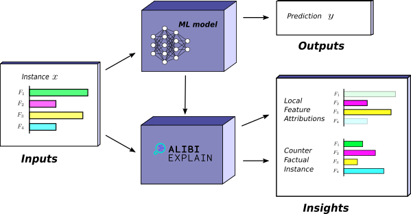
Alibi provides a set of algorithms or methods known as explainers. Each explainer provides some kind of insight about a model. The set of insights available given a trained model is dependent on a number of factors. For instance, if the model is a regression model it makes sense to ask how the prediction varies for some regressor. Whereas it doesn’t make sense to ask what minimal change is required to obtain a new class prediction. In general, given a model the explainers available from Alibi are constrained by:

• The type of data the model handles. Each insight applies to some or all of the following kinds of data: image, tabular or textual.

• The task the model performs. Alibi provides explainers for regression or classification models.

• The type of model used. Examples of model types include neural networks and random forests.

Applications

As machine learning methods have become more complex and more mainstream, with many industries now incorporating AI in some form or another, the need to understand the decisions made by models is only increasing. Explainability has several applications of importance.

• Trust: At a core level, explainability builds trust in the machine learning systems we use. It allows us to justify their use in many contexts where an understanding of the basis of the decision is paramount. This is a common issue within machine learning in medicine, where acting on a model prediction may require expensive or risky procedures to be carried out.

• Testing: Explainability might be used to audit financial models that aid decisions about whether to grant customer loans. By computing the attribution of each feature towards the prediction the model makes, organisations can check that they are consistent with human decision-making. Similarly, explainability applied to a model trained on image data can explicitly show the model’s focus when making decisions, aiding debugging. Practitioners must be wary of misuse, however.

• Functionality: Insights can be used to augment model functionality. For instance, providing information on top of model predictions such as how to change model inputs to obtain desired outputs.

• Research: Explainability allows researchers to understand how and why opaque models make decisions. This can help them understand more broadly the effects of the particular model or training schema they’re using.

Black-box vs White-box methods

Some explainers apply only to specific types of models such as the Tree SHAP methods which can only be used with tree-based models. This is the case when an explainer uses some aspect of that model’s internal structure. If the model is a neural network then some methods require taking gradients of the model predictions with respect to the inputs. Methods that require access to the model internals are known as white-box methods. Other explainers apply to any type of model. They can do so because the underlying method doesn’t make use of the model internals. Instead, they only need to have access to the model outputs given particular inputs. Methods that apply in this general setting are known as black-box methods. Typically, white-box methods are faster than black-box methods as they can exploit the model internals. For a more detailed discussion see white-box and black-box models.

Note 1: Black-box Definition

The use of black-box here varies subtly from the conventional use within machine learning. In most other contexts a model is a black-box if the mechanism by which it makes predictions is too complicated to be interpretable to a human. Here we use black-box to mean that the explainer method doesn’t need access to the model internals to be applied.

Global and Local Insights

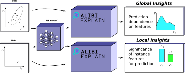
Insights can be categorised into two categories — local and global. Intuitively, a local insight says something about a single prediction that a model makes. For example, given an image classified as a cat by a model, a local insight might give the set of features (pixels) that need to stay the same for that image to remain classified as a cat.

On the other hand, global insights refer to the behaviour of the model over a range of inputs. As an example, a plot that shows how a regression prediction varies for a given feature. These insights provide a more general understanding of the relationship between inputs and model predictions.

Biases

The explanations Alibi’s methods provide depend on the model, the data, and — for local methods — the instance of interest. Thus Alibi allows us to obtain insight into the model and, therefore, also the data, albeit indirectly. There are several pitfalls of which the practitioner must be wary.

Often bias exists in the data we feed machine learning models even when we exclude sensitive factors. Ostensibly explainability is a solution to this problem as it allows us to understand the model’s decisions to check if they’re appropriate. However, human bias itself is still an element. Hence, if the model is doing what we expect it to on biased data, we are vulnerable to using explainability to justify relations in the data that may not be accurate. Consider:

“Before launching the model, risk analysts are asked to review the Shapley value explanations to ensure that the model exhibits expected behavior (i.e., the model uses the same features that a human would for the same task).” — Explainable Machine Learning in Deployment

The critical point here is that the risk analysts in the above scenario must be aware of their own bias and potential bias in the dataset. The Shapley value explanations themselves don’t remove this source of human error; they just make the model less opaque.

Machine learning engineers may also have expectations about how the model should be working. An explanation that doesn’t conform to their expectations may prompt them to erroneously decide that the model is “incorrect”. People usually expect classifiers trained on image datasets to use the same structures humans naturally do when identifying the same classes. However, there is no reason to believe such models should behave the same way we do.

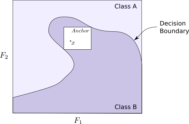
Interpretability of insights can also mislead. Some insights such as anchors give conditions for a classifiers prediction. Ideally, the set of these conditions would be small. However, when obtaining anchors close to decision boundaries, we may get a complex set of conditions to differentiate that instance from near members of a different class. Because this is harder to understand, one might write the model off as incorrect, while in reality, the model performs as desired.

Types of Insights

Alibi provides several local and global insights with which to explore and understand models. The following gives the practitioner an understanding of which explainers are suitable in which situations.

Explainer	Scope	Model types	Task types	Data types	Use	Resources
Accumulated Local Effects	Global	Black-box	Classification, Regression	Tabular (numerical)	How does model prediction vary with respect to features of interest?	docs, paper
Partial Dependence	Global	Black-box, White-box (scikit-learn)	Classification, Regression	Tabular (numerical, categorical)	How does model prediction vary with respect to features of interest?	docs, paper
Partial Dependence Variance	Global	Black-box, White-box (scikit-learn)	Classification, Regression	Tabular (numerical, categorical)	Which are the most important features globally? How much do features interact globally?	docs, paper
Permutation importance	Global	Black-box	Classification, Regression	Tabular (numerical, categorical)	Which are the most important features globally?	docs, paper
Anchors	Local	Black-box	Classification	Tabular (numerical, categorical), Text and Image	Which set of features of a given instance are sufficient to ensure the prediction stays the same?	docs, paper
Pertinent Positives	Local	Black-box, White-box (TensorFlow)	Classification	Tabular (numerical), Image	“”	docs, paper
Integrated Gradients	Local	White-box (TensorFlow)	Classification, Regression	Tabular (numerical, categorical), Text and Image	What does each feature contribute to the model prediction?	docs, paper
Kernel SHAP	Local	Black-box	Classification, Regression	Tabular (numerical, categorical)	“”	docs, paper
Tree SHAP (path-dependent)	Local	White-box (XGBoost, LightGBM, CatBoost, scikit-learn and pyspark tree models)	Classification, Regression	Tabular (numerical, categorical)	“”	docs, paper
Tree SHAP (interventional)	Local	White-box (XGBoost, LightGBM, CatBoost, scikit-learn and pyspark tree models)	Classification, Regression	Tabular (numerical, categorical)	“”	docs, paper
Counterfactual Instances	Local	Black-box (differentiable), White-box (TensorFlow)	Classification	Tabular (numerical), Image	What minimal change to features is required to reclassify the current prediction?	docs, paper
Contrastive Explanation Method	Local	Black-box (differentiable), White-box (TensorFlow)	Classification	Tabular (numerical), Image	“”	docs, paper
Counterfactuals Guided by Prototypes	Local	Black-box (differentiable), White-box (TensorFlow)	Classification	Tabular (numerical, categorical), Image	“”	docs, paper
Counterfactuals with Reinforcement Learning	Local	Black-box	Classification	Tabular (numerical, categorical), Image	“”	docs, paper
Similarity explanations	Local	White-box	Classification, Regression	Tabular (numerical, categorical), Text and Image	What are the instances in the training set that are most similar to the instance of interest according to the model?	docs, paper

1. Global Feature Attribution

Global Feature Attribution methods aim to show the dependency of model output on a subset of the input features. They provide global insight describing the model’s behaviour over the input space. For instance, Accumulated Local Effects plots obtain graphs that directly visualize the relationship between feature and prediction over a specific set of samples.

Suppose a trained regression model that predicts the number of bikes rented on a given day depending on the temperature, humidity, and wind speed. A global feature attribution plot for the temperature feature might be a line graph plotted against the number of bikes rented. One would anticipate an increase in rentals until a specific temperature and then a decrease after it gets too hot.

Accumulated Local Effects

Explainer	Scope	Model types	Task types	Data types	Use	Resources
Accumulated Local Effects	Global	Black-box	Classification, Regression	Tabular (numerical)	How does model prediction vary with respect to features of interest?	docs, paper

Alibi provides accumulated local effects (ALE) plots because they give the most accurate insight. Alternatives include Partial Dependence Plots (PDP), of which ALE is a natural extension. Suppose we have a model \(f\) and features \(X=\{x_1,... x_n\}\). Given a subset of the features \(X_S\), we denote \(X_C=X \setminus X_S\). \(X_S\) is usually chosen to be of size at most 2 in order to make the generated plots easy to visualize. PDP works by marginalizing the model’s output over the features we are not interested in, \(X_C\). The process of factoring out the \(X_C\) set causes the introduction of artificial data, which can lead to errors. ALE plots solve this by using the conditional probability distribution instead of the marginal distribution and removing any incorrect output dependencies due to correlated input variables by accumulating local differences in the model output instead of averaging them. See the following for a more expansive explanation.

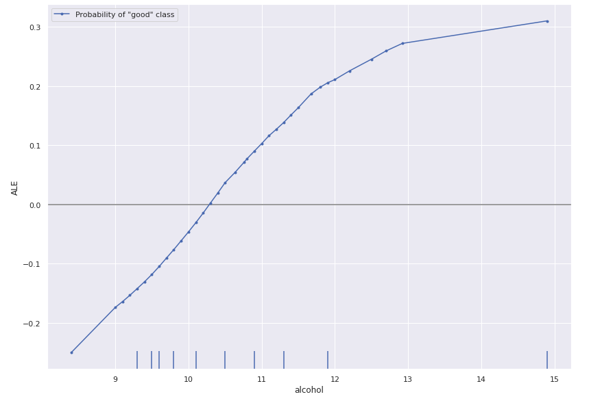
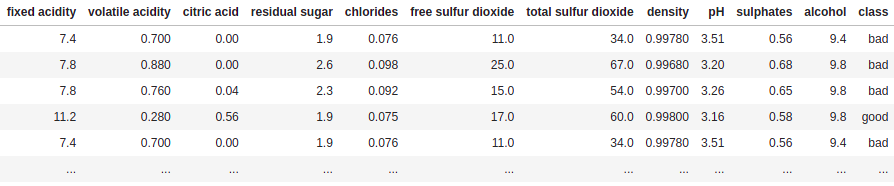
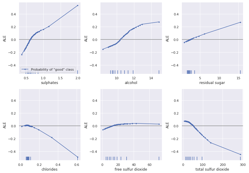
We illustrate the use of ALE on the wine-quality dataset which is a tabular numeric dataset with wine quality as the target variable. Because we want a classification task we split the data into good and bad classes using 5 as the threshold. We can compute the ALE with Alibi (see notebook) by simply using:

from alibi.explainers import ALE, plot_ale

# Model is a binary classifier so we only take the first model output corresponding to "good" class probability.
predict_fn = lambda x: model(scaler.transform(x)).numpy()[:, 0]
ale = ALE(predict_fn, feature_names=features)
exp = ale.explain(X_train)

# Plot the explanation for the "Alcohol feature"
plot_ale(exp, features=['alcohol'], line_kw={'label': 'Probability of "good" class'})

Hence, we see the model predicts higher alcohol content wines as being better:

Note 2: Categorical Variables and ALE

Note that while ALE is well-defined on numerical tabular data, it isn’t on categorical data. This is because it’s unclear what the difference between two categorical values should be. Note that if the dataset has a mix of categorical and numerical features, we can always compute the ALE of the numerical ones.

Pros	Cons
ALE plots are easy to visualize and understand intuitively	Harder to explain the underlying motivation behind the method than PDP plots or M plots
Very general as it is a black-box algorithm	Requires access to the training dataset
Doesn’t struggle with dependencies in the underlying features, unlike PD plots	ALE of categorical variables is not well-defined
ALE plots are fast

Partial Dependence

Explainer	Scope	Model types	Task types	Data types	Use	Resources
Partial Dependence	Global	Black-box, White-box (scikit-learn)	Classification, Regression	Tabular (numerical, categorical)	How does model prediction vary with respect to features of interest?	docs, paper

Alibi provides partial dependence (PD) plots as an alternative to ALE. Following the same notation as above, we remind the reader that the PD is marginalizing the model’s output over the features we are not interested in, \(X_C\). This approach has a direct extension for categorical features, something that ALE struggle with. Although, the practitioner should be aware of the main limitation of PD, which is the assumption of feature independence. The process of marginalizing out the set \(X_C\) under the assumption of feature independence might thus include in the computation predictions for data instances belonging to low probability regions of the features distribution.

Pros	Cons
PD plots are easy to visualize and understand intuitively (easier than ALE)	Struggle with dependencies in the underlying features. In the uncorrelated case the interpretation might be unclear.
Very general as it is a black-box algorithm	Heterogeneous effects might be hidden (ICE to the rescue)
PD plots are in general fast. Even faster implementation for scikit-learn tree based models
PD plots have causal interpretation. The relationship is causal for the model, but not necessarily for the real world
Natural extension to categorical features

Partial Dependence Variance

Explainer	Scope	Model types	Task types	Data types	Use	Resources
Partial Dependence Variance	Global	Black-box, White-box (scikit-learn)	Classification, Regression	Tabular (numerical, categorical)	What are the most important features globally? How much do features interact globally?	docs, paper

Alibi provides partial dependence variance as a way to measure globally the feature importance and the strength of the feature interactions between pairs of features. Since the method is based on the partial dependence, the practitioner should be aware that the method inherits its main limitations (see discussion above).

Pros	Cons
Intuitive motivation for the computation of the feature importance	The feature importance captures only the main effect and ignores possible feature interaction
Very general as it is a black-box algorithm	Can fail to detect feature interaction even though those exist
Fast computation in general. Even faster implementation for scikit-learn tree-based models
Offers standardized procedure to quantify the feature importance (i.e., contrasts with internal feature importance for some tree-based model)
Offers support for both numerical and categorical features
Can quantify the strength of potential interaction effects

Permutation Importance

Explainer	Scope	Model types	Task types	Data types	Use	Resources
Permutation Importance	Global	Black-box	Classification, Regression	Tabular (numerical, categorical)	Which are the most important features globally?	docs, paper

Alibi provides permutation importance as a way to measure globally the feature importance. The computation of the feature importance is based on the degree of model performance degradation when the feature values within a feature column are permuted. One important behavior that a practitioner should be aware of is that the importance of correlated features can be split between them.

Pros	Cons
A nice and simple interpretation - the feature importance is the increase/decrease in the model loss/score when a feature is noise.	Need the ground truth labels
Very general as it is a black-box algorithm	Can be biased towards unrealistic data instances
The feature importance takes into account all the feature interactions	The importance metric is related to the loss/score function
Does not require retraining the model

2. Local Necessary Features

Local necessary features tell us what features need to stay the same for a specific instance in order for the model to give the same classification. In the case of a trained image classification model, local necessary features for a given instance would be a minimal subset of the image that the model uses to make its decision. Alibi provides two explainers for computing local necessary features: anchors and pertinent positives.

Anchors

Explainer	Scope	Model types	Task types	Data types	Use	Resources
Anchors	Local	Black-box	Classification	Tabular (numerical, categorical), Text and Image	Which set of features of a given instance are sufficient to ensure the prediction stays the same?	docs, paper

Anchors are introduced in Anchors: High-Precision Model-Agnostic Explanations. More detailed documentation can be found here.

Let \(A\) be a rule (set of predicates) acting on input instances, such that \(A(x)\) returns \(1\) if all its feature predicates are true. Consider the wine quality dataset adjusted by partitioning the data into good and bad wine based on a quality threshold of 0.5:

An example of a predicate for this dataset would be a rule of the form: 'alcohol > 11.00'. Note that the more predicates we add to an anchor, the fewer instances it applies to, as by doing so, we filter out more instances of the data. Anchors are sets of predicates associated to a specific instance \(x\) such that \(x\) is in the anchor (\(A(x)=1\)) and any other point in the anchor has the same classification as \(x\) (\(z\) such that \(A(z) = 1 \implies f(z) = f(x)\) where \(f\) is the model). We’re interested in finding the Anchor that contains both the most instances and also \(x\).

To construct an anchor using Alibi for tabular data such as the wine quality dataset (see notebook), we use:

from alibi.explainers import AnchorTabular

predict_fn = lambda x: model.predict(scaler.transform(x))
explainer = AnchorTabular(predict_fn, features)
explainer.fit(X_train)

# x is the instance to explain
result = explainer.explain(x)

print('Anchor =', result.data['anchor'])
print('Coverage = ', result.data['coverage'])

where x is an instance of the dataset classified as good.

Mean test accuracy 95.00%
Anchor = ['sulphates <= 0.55', 'volatile acidity > 0.52', 'alcohol <= 11.00', 'pH > 3.40']
Coverage =  0.0316930775646372

Note: Alibi also gives an idea of the size (coverage) of the Anchor which is the proportion of the input space the anchor applies to.

To find anchors Alibi sequentially builds them by generating a set of candidates from an initial anchor candidate, picking the best candidate of that set and then using that to generate the next set of candidates and repeating. Candidates are favoured on the basis of the number of instances they contain that are in the same class as \(x\) under \(f\). The proportion of instances the anchor contains that are classified the same as \(x\) is known as the precision of the anchor. We repeat the above process until we obtain a candidate anchor with satisfactory precision. If there are multiple such anchors we choose the one that contains the most instances (as measured by coverage).

To compute which of two anchors is better, Alibi obtains an estimate by sampling from \(\mathcal{D}(z|A)\) where \(\mathcal{D}\) is the data distribution. The sampling process is dependent on the type of data. For tabular data, this process is easy; we can fix the values in the Anchor and replace the rest with values from points sampled from the dataset.

In the case of textual data, anchors are sets of words that the sentence must include to be in the anchor. To sample from \(\mathcal{D}(z|A)\), we need to find realistic sentences that include those words. To help do this Alibi provides support for three transformer based language models: DistilbertBaseUncased, BertBaseUncased, and RobertaBase.

Image data being high-dimensional means we first need to reduce it to a lower dimension. We can do this using image segmentation algorithms (Alibi supports felzenszwalb , slic and quickshift) to find super-pixels. The user can also use their own custom defined segmentation function. We then create the anchors from these super-pixels. To sample from \(\mathcal{D}(z|A)\) we replace those super-pixels that aren’t in \(A\) with something else. Alibi supports superimposing over the absent super-pixels with an image sampled from the dataset or taking the average value of the super-pixel.

The fact that the method requires perturbing and comparing anchors at each stage leads to some limitations. For instance, the more features, the more candidate anchors you can obtain at each process stage. The algorithm uses a beam search among the candidate anchors and solves for the best \(B\) anchors at each stage in the process by framing the problem as a multi-armed bandit. The runtime complexity is \(\mathcal{O}(B \cdot p^2 + p^2 \cdot \mathcal{O}_{MAB[B \cdot p, B]})\) where \(p\) is the number of features and \(\mathcal{O}_ {MAB[B \cdot p, B]}\) is the runtime for the multi-armed bandit ( see Molnar for more details).

Similarly, comparing anchors that are close to decision boundaries can require many samples to obtain a clear winner between the two. Also, note that anchors close to decision boundaries are likely to have many predicates to ensure the required predictive property. This makes them less interpretable.

Pros	Cons
Easy to explain as rules are simple to interpret	Time complexity scales as a function of features
Is a black-box method as we need to predict the value of an instance and don’t need to access model internals	Requires a large number of samples to distinguish anchors close to decision boundaries
The coverage of an anchor gives a level of global insight as well	Anchors close to decision boundaries are less likely to be interpretable
	High dimensional feature spaces such as images need to be reduced to improve the runtime complexity
	Practitioners may need domain-specific knowledge to correctly sample from the conditional probability

Contrastive Explanation Method (Pertinent Positives)

Explainer	Scope	Model types	Task types	Data types	Use	Resources
Pertinent Positives	Local	Black-box, White-box (TensorFlow)	Classification	Tabular (numerical), Image	Which set of features of a given instance is sufficient to ensure the prediction stays the same	docs, paper

Introduced by Amit Dhurandhar, et al, a Pertinent Positive is the subset of features of an instance that still obtains the same classification as that instance. These differ from anchors primarily in the fact that they aren’t constructed to maximize coverage. The method to create them is also substantially different. The rough idea is to define an absence of a feature and then perturb the instance to take away as much information as possible while still retaining the original classification. Note that these are a subset of the CEM method which is also used to construct pertinent negatives/counterfactuals.

Given an instance \(x\) we use gradient descent to find a \(\delta\) that minimizes the following loss:

\[ L = c\cdot L_{pred}(\delta) + \beta L_{1}(\delta, x) + L_{2}^{2}(\delta, x) + \gamma \|\delta - AE(\delta)\|^{2}_{2} \]

\(AE\) is an autoencoder generated from the training data. If \(\delta\) strays from the original data distribution, the autoencoder loss will increase as it will no longer reconstruct \(\delta\) well. Thus, we ensure that \(\delta\) remains close to the original dataset distribution.

Note that \(\delta\) is constrained to only “take away” features from the instance \(x\). There is a slightly subtle point here: removing features from an instance requires correctly defining non-informative feature values. For the MNIST digits, it’s reasonable to assume that the black background behind each digit represents an absence of information. In general, having to choose a non-informative value for each feature is non-trivial and domain knowledge is required. This is the reverse to the contrastive explanation method (pertinent-negatives) method introduced in the section on counterfactual instances.

Note that we need to compute the loss gradient through the model. If we have access to the internals, we can do this directly. Otherwise, we need to use numerical differentiation at a high computational cost due to the extra model calls we need to make. This does however mean we can use this method for a wide range of black-box models but not all. We require the model to be differentiable which isn’t always true. For instance tree-based models have piece-wise constant output.

Pros	Cons
Can be used with both white-box (TensorFlow) and some black-box models	Finding non-informative feature values to take away from an instance is often not trivial, and domain knowledge is essential
	The autoencoder loss requires access to the original dataset
	Need to tune hyperparameters \(\beta\) and \(\gamma\)
	The insight doesn’t tell us anything about the coverage of the pertinent positive
	Slow for black-box models due to having to numerically evaluate gradients
	Only works for differentiable black-box models

3. Local Feature Attribution

Local feature attribution (LFA) asks how each feature in a given instance contributes to its prediction. In the case of an image, this would highlight those pixels that are most responsible for the model prediction. Note that this differs subtly from Local Necessary Features which find the minimal subset of features required to keep the same prediction. Local feature attribution instead assigns a score to each feature.

A good example use of local feature attribution is to detect that an image classifier is focusing on the correct features of an image to infer the class. In their paper “Why Should I Trust You?”: Explaining the Predictions of Any Classifier, Marco Tulio Ribeiro et al. train a logistic regression classifier on a small dataset of images of wolves and huskies. The data set has been handpicked so that only the pictures of wolves have snowy backdrops while the huskies don’t. LFA methods reveal that the resulting misclassification of huskies in snow as wolves results from the network incorrectly focusing on those images snowy backdrops.

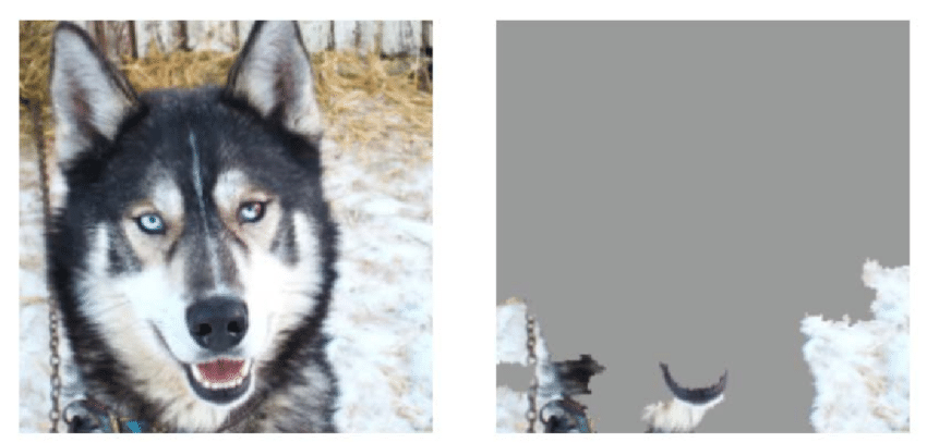
Figure 11 from “Why Should I Trust You?”: Explaining the Predictions of Any Classifier.

Let \(f:\mathbb{R}^n \rightarrow \mathbb{R}\). \(f\) might be a regression model, a single component of a multi-output regression or a probability of a class in a classification model. If \(x=(x_1,... ,x_n) \in \mathbb{R}^n\) then an attribution of the prediction at input \(x\) is a vector \(a=(a_1,... ,a_n) \in \mathbb{R}^n\) where \(a_i\) is the contribution of \(x_i\) to the prediction \(f(x)\).

Alibi exposes four explainers to compute LFAs: Integrated Gradients , Kernel SHAP , Path-dependent Tree SHAP and Interventional Tree SHAP. The last three of these are implemented in the SHAP library and Alibi acts as a wrapper. Interventional and path-dependent tree SHAP are white-box methods that apply to tree based models.

For attribution methods to be relevant, we expect the attributes to behave consistently in certain situations. Hence, they should satisfy the following properties.

• Efficiency/Completeness: The sum of attributions should equal the difference between the prediction and the baseline

• Symmetry: Variables that have identical effects on the model should have equal attribution

• Dummy/Sensitivity: Variables that don’t change the model output should have attribution zero

• Additivity/Linearity: The attribution of a feature for a linear combination of two models should equal the linear combination of attributions of that feature for each of those models

Not all LFA methods satisfy these methods (LIME for example) but the ones provided by Alibi (Integrated Gradients, Kernel SHAP , Path-dependent and Interventional Tree SHAP) do.

Integrated Gradients

Explainer	Scope	Model types	Task types	Data types	Use	Resources
Integrated Gradients	Local	White-box (TensorFlow)	Classification, Regression	Tabular (numerical, categorical), Text and Image	What does each feature contribute to the model prediction?	docs, paper

The Integrated Gradients (IG) method computes the attribution of each feature by integrating the model partial derivatives along a path from a baseline point to the instance. This accumulates the changes in the prediction that occur due to the changing feature values. These accumulated values represent how each feature contributes to the prediction for the instance of interest. A more detailed explanation of the method can be found in the method specific docs.

We need to choose a baseline which should capture a blank state in which the model makes essentially no prediction or assigns the probability of each class equally. This is dependent on domain knowledge of the dataset. In the case of MNIST for instance a common choice is an image set to black. For numerical tabular data we can set the baseline as the average of each feature.

Note 3: Choice of Baseline

The main difficulty with this method is that as IG is very dependent on the baseline, it’s essential to make sure you choose it well. Choosing a black image baseline for a classifier trained to distinguish between photos taken at day or night may not be the best choice.

Note that IG is a white-box method that requires access to the model internals in order to compute the partial derivatives. Alibi provides support for TensorFlow models. For example given a TensorFlow classifier trained on the wine quality dataset we can compute the IG attributions (see notebook) by doing:

from alibi.explainers import IntegratedGradients

ig = IntegratedGradients(model)   # TensorFlow model
result = ig.explain(
  scaler.transform(x),            # scaled data instance 
  target=0,                       # model class probability prediction to obtain attribution for 
)

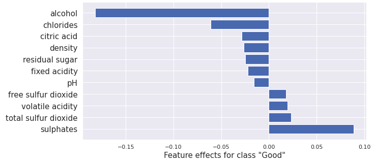
plot_importance(result.data['attributions'][0], features, 0)

This gives:

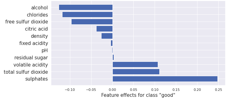
Note 4: Comparison to ALE

The alcohol feature value contributes negatively here to the “Good” prediction which seems to contradict the ALE result. However, The instance \(x\) we choose has an alcohol content of 9.4%, which is reasonably low for a wine classed as “Good” and is consistent with the ALE plot. (The median for good wines is 10.8% and bad wines 9.7%)

Pros	Cons
Simple to understand and visualize, especially with image data	White-box method. Requires the partial derivatives of the model outputs with respect to inputs
Doesn’t require access to the training data	Requires choosing the baseline which can have a significant effect on the outcome
Satisfies several desirable properties

Kernel SHAP

Explainer	Scope	Model types	Task types	Data types	Use	Resources
Kernel SHAP	Local	Black-box	Classification, Regression	Tabular (numerical, categorical)	What does each feature contribute to the model prediction?	docs, paper

Kernel SHAP (Alibi method docs) is a method for computing the Shapley values of a model around an instance. Shapley values are a game-theoretic method of assigning payout to players depending on their contribution to an overall goal. In our case, the features are the players, and the payouts are the attributions.

Given any subset of features, we can ask how a feature’s presence in that set contributes to the model output. We do this by computing the model output for the set with and without the specific feature. We obtain the Shapley value for that feature by considering these contributions with and without it present for all possible subsets of features.

Two problems arise. Most models are not trained to take a variable number of input features. And secondly, considering all possible sets of absent features leads to considering the power set which is prohibitively large when there are many features.

To solve the former, we sample from the interventional conditional expectation. This replaces missing features with values sampled from the training distribution. And to solve the latter, the kernel SHAP method samples on the space of subsets to obtain an estimate.

A downside of interfering in the distribution like this is that doing so introduces unrealistic samples if there are dependencies between the features.

Alibi provides a wrapper to the SHAP library. We can use this explainer to compute the Shapley values for a sklearn random forest model using the following (see notebook):

from alibi.explainers import KernelShap

# black-box model
predict_fn = lambda x: rfc.predict_proba(scaler.transform(x))
explainer = KernelShap(predict_fn, task='classification')
explainer.fit(X_train[0:100])
result = explainer.explain(x)

plot_importance(result.shap_values[1], features, 1)

This gives the following output:

This result is similar to the one for Integrated Gradients although there are differences due to using different methods and models in each case.

Pros	Cons
Satisfies several desirable properties	Kernel SHAP is slow owing to the number of samples required to estimate the Shapley values accurately
Shapley values can be easily interpreted and visualized	The interventional conditional probability introduces unrealistic data points
Very general as is a black-box method	Requires access to the training dataset

Path-dependent Tree SHAP

Explainer	Scope	Model types	Task types	Data types	Use	Resources
Tree SHAP (path-dependent)	Local	White-box (XGBoost, LightGBM, CatBoost, scikit-learn and pyspark tree models)	Classification, Regression	Tabular (numerical, categorical)	What does each feature contribute to the model prediction?	docs, paper

Computing the Shapley values for a model requires computing the interventional conditional expectation for each member of the power set of instance features. For tree-based models we can approximate this distribution by applying the tree as usual. However, for missing features, we take both routes down the tree, weighting each path taken by the proportion of samples from the training dataset that go each way. The tree SHAP method does this simultaneously for all members of the feature power set, obtaining a significant speedup . Assume the random forest has \(T\) trees, with a depth of \(D\), let \(L\) be the number of leaves and let \(M\) be the size of the feature set. If we compute the approximation for each member of the power set we obtain a time complexity of \(O( TL2^M)\). In contrast, computing for all sets simultaneously we achieve \(O(TLD^2)\).

To compute the path-dependent tree SHAP explainer for a random forest using Alibi ( see notebook) we use:

from alibi.explainers import TreeShap

# rfc is a random forest model
path_dependent_explainer = TreeShap(rfc)
path_dependent_explainer.fit()                                  # path dependent Tree SHAP doesn't need any data

result = path_dependent_explainer.explain(scaler.transform(x))  # explain the scaled instance
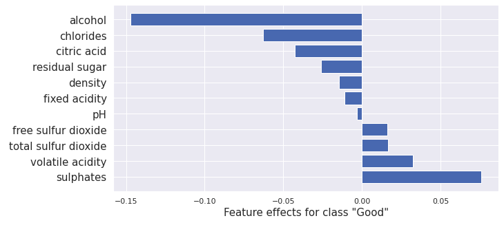
plot_importance(result.shap_values[1], features, '"Good"')

From this we obtain:

This result is similar to the one for Integrated Gradients and Kernel SHAP although there are differences due to using different methods and models in each case.

Pros	Cons
Satisfies several desirable properties	Only applies to tree-based models
Very fast for a valuable category of models	Uses an approximation of the interventional conditional expectation instead of computing it directly
Doesn’t require access to the training data
Shapley values can be easily interpreted and visualized

Interventional Tree SHAP

Explainer	Scope	Model types	Task types	Data types	Use	Resources
Tree SHAP (interventional)	Local	White-box (XGBoost, LightGBM, CatBoost, scikit-learn and pyspark tree models)	Classification, Regression	Tabular (numerical, categorical)	What does each feature contribute to the model prediction?	docs, paper

Suppose we sample a reference data point, \(r\), from the training dataset. Let \(F\) be the set of all features. For each feature, \(i\), we then enumerate over all subsets of \(S\subset F \setminus \{i\}\). If a subset is missing a feature, we replace it with the corresponding one in the reference sample. We can then compute \(f(S)\) directly for each member of the power set of instance features to get the Shapley values.

Enforcing independence of the \(S\) and \(F\setminus S\) in this way is known as intervening in the underlying data distribution and is the source of the algorithm’s name. Note that this breaks any independence between features in the dataset, which means the data points we’re sampling won’t always be realistic.

For a single tree and sample \(r\) if we iterate over all the subsets of \(S \subset F \setminus \{i\}\), it would give \(O( M2^M)\) time complexity. The interventional tree SHAP algorithm runs with \(O(TLD)\) time complexity.

The main difference between the interventional and the path-dependent tree SHAP methods is that the latter approximates the interventional conditional expectation, whereas the former method calculates it directly.

To compute the interventional tree SHAP explainer for a random forest using Alibi ( see notebook), we use:

from alibi.explainers import TreeShap

# rfc is a random forest classifier model
tree_explainer_interventional = TreeShap(rfc)

# interventional tree SHAP is slow for large datasets so we take first 100 samples of training data.
tree_explainer_interventional.fit(scaler.transform(X_train[0:100]))

result = tree_explainer_interventional.explain(scaler.transform(x))  # explain the scaled instance
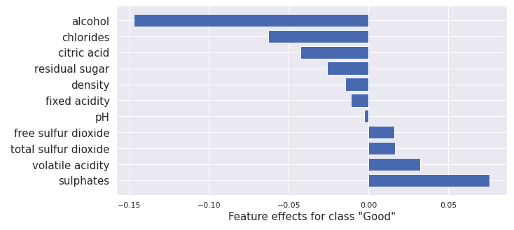
plot_importance(result.shap_values[1], features, '"Good"')

From this we obtain:

This result is similar to the one for Integrated Gradients, Kernel SHAP , Path-dependent Tree SHAP although there are differences due to using different methods and models in each case.

For a great interactive explanation of the interventional Tree SHAP method see.

Pros	Cons
Satisfies several desirable properties	Only applies to tree-based models
Very fast for a valuable category of models	Requires access to the dataset
Shapley values can be easily interpreted and visualized	Typically slower than the path-dependent method
Computes the interventional conditional expectation exactly unlike the path-dependent method

4. Counterfactual instances

Given an instance of the dataset and a prediction given by a model, a question naturally arises how would the instance minimally have to change for a different prediction to be provided. Such a generated instance is known as a counterfactual. Counterfactuals are local explanations as they relate to a single instance and model prediction.

Given a classification model trained on the MNIST dataset and a sample from the dataset, a counterfactual would be a generated image that closely resembles the original but is changed enough that the model classifies it as a different number from the original instance.

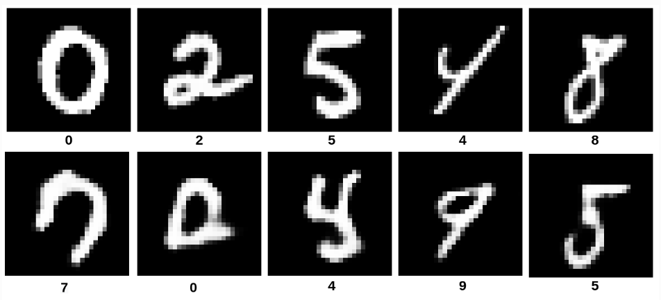
From Samoilescu RF et al., Model-agnostic and Scalable Counterfactual Explanations via Reinforcement Learning, 2021

Counterfactuals can be used to both debug and augment model functionality. Given tabular data that a model uses to make financial decisions about a customer, a counterfactual would explain how to change their behavior to obtain a different conclusion. Alternatively, it may tell the Machine Learning Engineer that the model is drawing incorrect assumptions if the recommended changes involve features that are irrelevant to the given decision. However, practitioners must still be wary of bias.

A counterfactual, \(x_{\text{cf}}\), needs to satisfy

• The model prediction on \(x_{\text{cf}}\) needs to be close to the pre-defined output (e.g. desired class label).

• The counterfactual \(x_{\text{cf}}\) should be interpretable.

The first requirement is clear. The second, however, requires some idea of what interpretable means. Alibi exposes four methods for finding counterfactuals: counterfactual instances (CFI) , contrastive explanations (CEM) , counterfactuals guided by prototypes (CFP), and counterfactuals with reinforcement learning (CFRL). Each of these methods deals with interpretability slightly differently. However, all of them require sparsity of the solution. This means we prefer to only change a small subset of the features which limits the complexity of the solution making it more understandable.

Note that sparse changes to the instance of interest doesn’t guarantee that the generated counterfactual is believably a member of the data distribution. CEM , CFP, and CFRL also require that the counterfactual be in distribution in order to be interpretable.

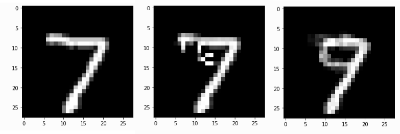
Original MNIST 7 instance, Counterfactual instances constructed using 1) counterfactual instances method, 2) counterfactual instances with prototypes method

The first three methods CFI , CEM , CFP all construct counterfactuals using a very similar method. They build them by defining a loss that prefer interpretable instances close to the target class. They then use gradient descent to move within the feature space until they obtain a counterfactual of sufficient quality. The main difference is the CEM and CFP methods also train an autoencoder to ensure that the constructed counterfactuals are within the data-distribution.

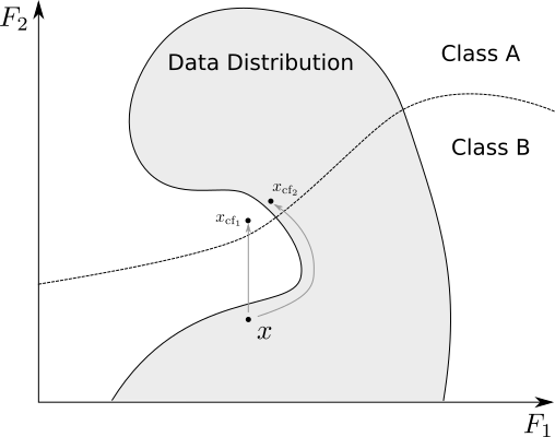
Obtaining counterfactuals using gradient descent with and without autoencoder trained on data distribution

These three methods only realistically work for grayscale images and anything multi-channel will not be interpretable. In order to get quality results for multi-channel images practitioners should use CFRL.

CFRL uses a similar loss to CEM and CFP but applies reinforcement learning to train a model which will generate counterfactuals on demand.

Note 5: fit and explain method runtime differences

Alibi explainers expose two methods, fit and explain. Typically in machine learning the method that takes the most time is the fit method, as that’s where the model optimization conventionally takes place. In explainability, the explain step often requires the bulk of computation. However, this isn’t always the case.

Among the explainers in this section, there are two approaches taken. The first finds a counterfactual when the user requests the insight. This happens during the .explain() method call on the explainer class. This is done by running gradient descent on model inputs to find a counterfactual. The methods that take this approach are counterfactual instances, contrastive explanation, and counterfactuals guided by prototypes. Thus, the fit method in these cases is quick, but the explain method is slow.

The other approach, counterfactuals with reinforcement learning, trains a model that produces explanations on demand. The training takes place during the fit method call, so this has a long runtime while the explain method is quick. If you want performant explanations in production environments, then the latter approach is preferable.

Counterfactual Instances

Explainer	Scope	Model types	Task types	Data types	Use	Resources
Counterfactual Instances	Local	Black-box (differentiable), White-box (TensorFlow)	Classification	Tabular(numerical), Image	What minimal change to features is required to reclassify the current prediction?	docs, paper

Let the model be given by \(f\), and let \(p_t\) be the target probability of class \(t\). Let \(\lambda\) be a hyperparameter. This method constructs counterfactual instances from an instance \(X\) by running gradient descent on a new instance \(X'\) to minimize the following loss:

\[L(X', X)= (f_{t}(X') - p_{t})^2 + \lambda L_{1}(X', X)\]

The first term pushes the constructed counterfactual towards the desired class, and the use of the \(L_{1}\) norm encourages sparse solutions.

This method requires computing gradients of the loss in the model inputs. If we have access to the model and the gradients are available, this can be done directly. If not, we can use numerical gradients, although this comes at a considerable performance cost.

A problem arises here in that encouraging sparse solutions doesn’t necessarily generate interpretable counterfactuals. This happens because the loss doesn’t prevent the counterfactual solution from moving off the data distribution. Thus, you will likely get an answer that doesn’t look like something that you would expect to see from the data.

To use the counterfactual instances method from Alibi applied to the wine quality dataset (see notebook), use:

from alibi.explainers import Counterfactual

explainer = Counterfactual(
    model,                              # The model to explain
    shape=(1,) + X_train.shape[1:],     # The shape of the model input
    target_proba=0.51,                  # The target class probability
    tol=0.01,                           # The tolerance for the loss
    target_class='other',               # The target class to obtain  
)

result_cf = explainer.explain(scaler.transform(x))
print("Instance prediction:", model.predict(scaler.transform(x))[0].argmax())
print("Counterfactual prediction:", model.predict(result_cf.data['cf']['X'])[0].argmax())

Gives the expected result:

Instance prediction: 0        # "good"
Counterfactual prediction: 1  # "bad"

Pros	Cons
Both a black-box and white-box method	Not likely to give human interpretable instances
Doesn’t require access to the training dataset	Requires tuning of \(\lambda\) hyperparameter
	Slow for black-box models due to having to numerically evaluate gradients

Contrastive Explanation Method (Pertinent Negatives)

Explainer	Scope	Model types	Task types	Data types	Use	Resources
Contrastive Explanation Method	Local	Black-box (differentiable), White-box (TensorFlow)	Classification	Tabular(numerical), Image	What minimal change to features is required to reclassify the current prediction?	docs, paper

CEM follows a similar approach to the above but includes three new details. Firstly an elastic net \(\beta L_{1} + L_{2}\) regularizer term is added to the loss. This term causes the solutions to be both close to the original instance and sparse.

Secondly, we require that \(\delta\) only adds new features rather than takes them away. We need to define what it means for a feature to be present so that the perturbation only works to add and not remove them. In the case of the MNIST dataset, an obvious choice of “present” feature is if the pixel is equal to 1 and absent if it is equal to 0. This is simple in the case of the MNIST data set but more difficult in complex domains such as colour images.

Thirdly, by training an autoencoder to penalize counterfactual instances that deviate from the data distribution. This works by minimizing the reconstruction loss of the autoencoder applied to instances. If a generated instance is unlike anything in the dataset, the autoencoder will struggle to recreate it well, and its loss term will be high. We require three hyperparameters \(c\), \(\beta\) and \(\gamma\) to define the following loss:

\[ L = c\cdot L_{pred}(\delta) + \beta L_{1}(\delta, x) + L_{2}^{2}(\delta, x) + \gamma \|\delta - AE(\delta)\|^{2}_{2} \]

A subtle aspect of this method is that it requires defining the absence or presence of features as delta is restrained only to allow you to add information. For the MNIST digits, it’s reasonable to assume that the black background behind each written number represents an absence of information. Similarly, in the case of colour images, you might take the median pixel value to convey no information, and moving away from this value adds information. For numerical tabular data, we can use the feature mean. In general, choosing a non-informative value for each feature is non-trivial, and domain knowledge is required. This is the reverse process to the contrastive explanation method (pertinent-positives) method introduced in the section on local necessary features in which we take away features rather than add them.

This approach extends the definition of interpretable to include a requirement that the computed counterfactual be believably a member of the dataset. This isn’t always satisfied (see image below). In particular, the constructed counterfactual often doesn’t look like a member of the target class.

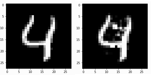
An original MNIST instance and a pertinent negative obtained using CEM.

To compute a pertinent-negative using Alibi (see notebook) we use:

from alibi.explainers import CEM

cem = CEM(model,                            # model to explain
          shape=(1,) + X_train.shape[1:],   # shape of the model input
          mode='PN',                        # pertinant negative mode
          kappa=0.2,                        # Confidence parameter for the attack loss term
          beta=0.1,                         # Regularization constant for L1 loss term
          ae_model=ae                       # autoencoder model
)

cem.fit(
    scaler.transform(X_train), # scaled training data
    no_info_type='median'      # non-informative value for each feature
)
result_cem = cem.explain(scaler.transform(x), verbose=False)
cem_cf = result_cem.data['PN']

print("Instance prediction:", model.predict(scaler.transform(x))[0].argmax())
print("Counterfactual prediction:", model.predict(cem_cf)[0].argmax())

Gives the expected result:

Instance prediction: 0        # "good"
Counterfactual prediction: 1  # "bad"

This method can apply to both black-box and white-box models. There is a performance cost from computing the numerical gradients in the black-box case due to having to numerically evaluate gradients.

Pros	Cons
Provides more interpretable instances than the counterfactual instances’ method.	Requires access to the dataset to train the autoencoder
Applies to both white and black-box models	Requires setup and configuration in choosing \(c\), \(\gamma\) and \(\beta\)
	Requires training an autoencoder
	Requires domain knowledge when choosing what it means for a feature to be present or not
	Slow for black-box models

Counterfactuals Guided by Prototypes

Explainer	Scope	Model types	Task types	Data types	Use	Resources
Counterfactuals Guided by Prototypes	Local	Black-box (differentiable), White-box (TensorFlow)	Classification	Tabular (numerical, categorical), Image	What minimal change to features is required to reclassify the current prediction?	docs, paper

For this method, we add another term to the loss that optimizes for the distance between the counterfactual instance and representative members of the target class. In doing this, we require interpretability also to mean that the generated counterfactual is believably a member of the target class and not just in the data distribution.

With hyperparameters \(c\), \(\gamma\) and \(\beta\), the loss is given by:

\[ L(X'|X)= c\cdot L_{pred}(X') + \beta L_{1}(X', X) + L_{2}(X', X)^2 + \gamma L_{2} (X', AE(X'))^2 + L_{2}(X', X_ {proto}) \]

This method produces much more interpretable results than CFI and CEM.

Because the prototype term steers the solution, we can remove the prediction loss term. This makes this method much faster if we are using a black-box model as we don’t need to compute the gradients numerically. However, occasionally the prototype isn’t a member of the target class. In this case you’ll end up with an incorrect counterfactual.

To use the counterfactual with prototypes method in Alibi (see notebook) we do:

from alibi.explainers import CounterfactualProto

explainer = CounterfactualProto(
    model,                           # The model to explain
    shape=(1,) + X_train.shape[1:],  # shape of the model input
    ae_model=ae,                     # The autoencoder
    enc_model=ae.encoder             # The encoder
)

explainer.fit(scaler.transform(X_train)) # Fit the explainer with scaled data

result_proto = explainer.explain(scaler.transform(x), verbose=False)

proto_cf = result_proto.data['cf']['X']
print("Instance prediction:", model.predict(scaler.transform(x))[0].argmax())
print("Counterfactual prediction:", model.predict(proto_cf)[0].argmax())

We get the following results:

Instance prediction: 0        # "good"
Counterfactual prediction: 1  # "bad"

Pros	Cons
Generates more interpretable instances than the CEM method	Requires access to the dataset
Black-box version of the method is fast	Requires setup and configuration in choosing \(\gamma\), \(\beta\) and \(c\)
Applies to more data-types	Requires training an autoencoder

Counterfactuals with Reinforcement Learning

Explainer	Scope	Model types	Task types	Data types	Use	Resources
Counterfactuals with Reinforcement Learning	Local	Black-box	Classification	Tabular (numerical, categorical), Image	What minimal change to features is required to reclassify the current prediction?	docs, paper

This black-box method splits from the approach taken by the above three significantly. Instead of minimizing a loss during the explain method call, it trains a new model when fitting the explainer called an actor that takes instances and produces counterfactuals. It does this using reinforcement learning. In reinforcement learning, an actor model takes some state as input and generates actions; in our case, the actor takes an instance with a target classification and attempts to produce a member of the target class. Outcomes of actions are assigned rewards dependent on a reward function designed to encourage specific behaviors. In our case, we reward correctly classified counterfactuals generated by the actor. As well as this, we reward counterfactuals that are close to the data distribution as modeled by an autoencoder. Finally, we require that they are sparse perturbations of the original instance. The reinforcement training step pushes the actor to take high reward actions. CFRL is a black-box method as the process by which we update the actor to maximize the reward only requires estimating the reward via sampling the counterfactuals.

As well as this, CFRL actors can be trained to ensure that certain constraints can be taken into account when generating counterfactuals. This is highly desirable as a use case for counterfactuals is to suggest the necessary changes to an instance to obtain a different classification. In some cases, you want these changes to be constrained, for instance, when dealing with immutable characteristics. In other words, if you are using the counterfactual to advise changes in behavior, you want to ensure the changes are enactable. Suggesting that someone needs to be two years younger to apply for a loan isn’t very helpful.

The training process requires randomly sampling data instances, along with constraints and target classifications. We can then compute the reward and update the actor to maximize it. We do this without needing access to the model internals; we only need to obtain a prediction in each case. The end product is a model that can generate interpretable counterfactual instances at runtime with arbitrary constraints.

To use CFRL on the wine dataset (see notebook), we use:

from alibi.explainers import CounterfactualRL 

predict_fn = lambda x: model(x)

cfrl_explainer = CounterfactualRL(
    predictor=predict_fn,               # The model to explain
    encoder=ae.encoder,                 # The encoder
    decoder=ae.decoder,                 # The decoder
    latent_dim=7,                       # The dimension of the autoencoder latent space
    coeff_sparsity=0.5,                 # The coefficient of sparsity
    coeff_consistency=0.5,              # The coefficient of consistency
    train_steps=10000,                  # The number of training steps
    batch_size=100,                     # The batch size
)

cfrl_explainer.fit(X=scaler.transform(X_train))

result_cfrl = cfrl_explainer.explain(X=scaler.transform(x), Y_t=np.array([1]))
print("Instance prediction:", model.predict(scaler.transform(x))[0].argmax())
print("Counterfactual prediction:", model.predict(result_cfrl.data['cf']['X'])[0].argmax())

Which gives the following output:

Instance prediction: 0        # "good"
Counterfactual prediction: 1  # "bad"

Note 6: CFRL explainers

Alibi exposes two explainer methods for counterfactuals with reinforcement learning. The first is the CounterfactualRL and the second is CounterfactualRlTabular. The difference is that CounterfactualRlTabular is designed to support categorical features. See the CFRL documentation page for more details.

Pros	Cons
Generates more interpretable instances than the CEM method	Longer to fit the model
Very fast at runtime	Requires to fit an autoencoder
Can be trained to account for arbitrary constraints	Requires access to the training dataset
General as is a black-box algorithm

Counterfactual Example Results

For each of the four explainers, we have generated a counterfactual instance. We compare the original instance to each:

Feature	Instance	CFI	CEM	CFP	CFRL
sulphates	0.67	0.64	0.549	0.623	0.598
alcohol	10.5	9.88	9.652	9.942	9.829
residual sugar	1.6	1.582	1.479	1.6	2.194
chlorides	0.062	0.061	0.057	0.062	0.059
free sulfur dioxide	5.0	4.955	2.707	5.0	6.331
total sulfur dioxide	12.0	11.324	12.0	12.0	14.989
fixed acidity	9.2	9.23	9.2	9.2	8.965
volatile acidity	0.36	0.36	0.36	0.36	0.349
citric acid	0.34	0.334	0.34	0.34	0.242
density	0.997	0.997	0.997	0.997	0.997
pH	3.2	3.199	3.2	3.2	3.188

The CFI, CEM, and CFRL methods all perturb more features than CFP, making them less interpretable. Looking at the ALE plots, we can see how the counterfactual methods change the features to flip the prediction. In general, each method seems to decrease the sulphates and alcohol content to obtain a “bad” classification consistent with the ALE plots. Note that the ALE plots potentially miss details local to individual instances as they are global insights.

5. Similarity explanations

Explainer	Scope	Model types	Task types	Data types	Use	Resources
Similarity explanations	Local	White-box	Classification, Regression	Tabular (numerical, categorical), Text and Image	What are the instances in the training set that are most similar to the instance of interest according to the model?	docs, paper

Similarity explanations are instance-based explanations that focus on training data points to justify a model prediction on a test instance. Given a trained model and a test instance whose prediction is to be explained, these methods scan the training set, finding the most similar data points according to the model which forms an explanation. This type of explanation can be interpreted as the model justifying its prediction by referring to similar instances which may share the same prediction—“I classify this image as a ‘Golden Retriever’ because it is most similar to images in the training set which I also classified as ‘Golden Retriever’”.

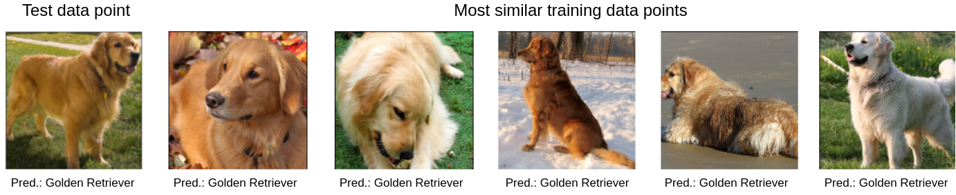
A similarity explanation justifies the classification of an image as a ‘Golden Retriever’ because most similar instances in the training set are also classified as ‘Golden Retriever’.