This page was generated from examples/cf_mnist.ipynb.
Counterfactual instances on MNIST
Given a test instance \(X\), this method can generate counterfactual instances \(X^\prime\) given a desired counterfactual class \(t\) which can either be a class specified upfront or any other class that is different from the predicted class of \(X\).
The loss function for finding counterfactuals is the following:
The first loss term, guides the search towards instances \(X^\prime\) for which the predicted class probability \(f_t(X^\prime)\) is close to a pre-specified target class probability \(p_t\) (typically \(p_t=1\)). The second loss term ensures that the counterfactuals are close in the feature space to the original test instance.
In this notebook we illustrate the usage of the basic counterfactual algorithm on the MNIST dataset.
Note
To enable support for Counterfactual, you may need to run
pip install alibi[tensorflow]
[1]:
import tensorflow as tf
tf.get_logger().setLevel(40) # suppress deprecation messages
tf.compat.v1.disable_v2_behavior() # disable TF2 behaviour as alibi code still relies on TF1 constructs
from tensorflow.keras.layers import Conv2D, Dense, Dropout, Flatten, MaxPooling2D, Input
from tensorflow.keras.models import Model, load_model
from tensorflow.keras.utils import to_categorical
import matplotlib
%matplotlib inline
import matplotlib.pyplot as plt
import numpy as np
import os
from time import time
from alibi.explainers import Counterfactual
print('TF version: ', tf.__version__)
print('Eager execution enabled: ', tf.executing_eagerly()) # False
TF version:  2.2.0
Eager execution enabled:  False
Load and prepare MNIST data
[2]:
(x_train, y_train), (x_test, y_test) = tf.keras.datasets.mnist.load_data()
print('x_train shape:', x_train.shape, 'y_train shape:', y_train.shape)
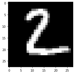
plt.gray()
plt.imshow(x_test[1]);
x_train shape: (60000, 28, 28) y_train shape: (60000,)
Prepare data: scale, reshape and categorize
[3]:
x_train = x_train.astype('float32') / 255
x_test = x_test.astype('float32') / 255
x_train = np.reshape(x_train, x_train.shape + (1,))
x_test = np.reshape(x_test, x_test.shape + (1,))
print('x_train shape:', x_train.shape, 'x_test shape:', x_test.shape)
y_train = to_categorical(y_train)
y_test = to_categorical(y_test)
print('y_train shape:', y_train.shape, 'y_test shape:', y_test.shape)
x_train shape: (60000, 28, 28, 1) x_test shape: (10000, 28, 28, 1)
y_train shape: (60000, 10) y_test shape: (10000, 10)
[4]:
xmin, xmax = -.5, .5
x_train = ((x_train - x_train.min()) / (x_train.max() - x_train.min())) * (xmax - xmin) + xmin
x_test = ((x_test - x_test.min()) / (x_test.max() - x_test.min())) * (xmax - xmin) + xmin
Define and train CNN model
[5]:
def cnn_model():
    x_in = Input(shape=(28, 28, 1))
    x = Conv2D(filters=64, kernel_size=2, padding='same', activation='relu')(x_in)
    x = MaxPooling2D(pool_size=2)(x)
    x = Dropout(0.3)(x)

    x = Conv2D(filters=32, kernel_size=2, padding='same', activation='relu')(x)
    x = MaxPooling2D(pool_size=2)(x)
    x = Dropout(0.3)(x)

    x = Flatten()(x)
    x = Dense(256, activation='relu')(x)
    x = Dropout(0.5)(x)
    x_out = Dense(10, activation='softmax')(x)

    cnn = Model(inputs=x_in, outputs=x_out)
    cnn.compile(loss='categorical_crossentropy', optimizer='adam', metrics=['accuracy'])

    return cnn
[6]:
cnn = cnn_model()
cnn.summary()
cnn.fit(x_train, y_train, batch_size=64, epochs=3, verbose=0)
cnn.save('mnist_cnn.h5')
Model: "model"
_________________________________________________________________
Layer (type)                 Output Shape              Param #
=================================================================
input_1 (InputLayer)         [(None, 28, 28, 1)]       0
_________________________________________________________________
conv2d (Conv2D)              (None, 28, 28, 64)        320
_________________________________________________________________
max_pooling2d (MaxPooling2D) (None, 14, 14, 64)        0
_________________________________________________________________
dropout (Dropout)            (None, 14, 14, 64)        0
_________________________________________________________________
conv2d_1 (Conv2D)            (None, 14, 14, 32)        8224
_________________________________________________________________
max_pooling2d_1 (MaxPooling2 (None, 7, 7, 32)          0
_________________________________________________________________
dropout_1 (Dropout)          (None, 7, 7, 32)          0
_________________________________________________________________
flatten (Flatten)            (None, 1568)              0
_________________________________________________________________
dense (Dense)                (None, 256)               401664
_________________________________________________________________
dropout_2 (Dropout)          (None, 256)               0
_________________________________________________________________
dense_1 (Dense)              (None, 10)                2570
=================================================================
Total params: 412,778
Trainable params: 412,778
Non-trainable params: 0
_________________________________________________________________
Evaluate the model on test set
[7]:
cnn = load_model('mnist_cnn.h5')
score = cnn.evaluate(x_test, y_test, verbose=0)
print('Test accuracy: ', score[1])
Test accuracy: 0.9871
Generate counterfactuals
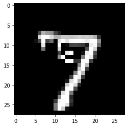
Original instance:
[8]:
X = x_test[0].reshape((1,) + x_test[0].shape)
plt.imshow(X.reshape(28, 28));

Counterfactual parameters:
[9]:
shape = (1,) + x_train.shape[1:]
target_proba = 1.0
tol = 0.01 # want counterfactuals with p(class)>0.99
target_class = 'other' # any class other than 7 will do
max_iter = 1000
lam_init = 1e-1
max_lam_steps = 10
learning_rate_init = 0.1
feature_range = (x_train.min(),x_train.max())
Run counterfactual:
[10]:
# initialize explainer
cf = Counterfactual(cnn, shape=shape, target_proba=target_proba, tol=tol,
                    target_class=target_class, max_iter=max_iter, lam_init=lam_init,
                    max_lam_steps=max_lam_steps, learning_rate_init=learning_rate_init,
                    feature_range=feature_range)

start_time = time()
explanation = cf.explain(X)
print('Explanation took {:.3f} sec'.format(time() - start_time))
Explanation took 8.407 sec
Results:
[11]:
pred_class = explanation.cf['class']
proba = explanation.cf['proba'][0][pred_class]

print(f'Counterfactual prediction: {pred_class} with probability {proba}')
plt.imshow(explanation.cf['X'].reshape(28, 28));
Counterfactual prediction: 9 with probability 0.9924006462097168
The counterfactual starting from a 7 moves towards the closest class as determined by the model and the data - in this case a 9. The evolution of the counterfactual during the iterations over \(\lambda\) can be seen below (note that all of the following examples satisfy the counterfactual condition):
[12]:
n_cfs = np.array([len(explanation.all[iter_cf]) for iter_cf in range(max_lam_steps)])
examples = {}
for ix, n in enumerate(n_cfs):
    if n>0:
        examples[ix] = {'ix': ix, 'lambda': explanation.all[ix][0]['lambda'],
                       'X': explanation.all[ix][0]['X']}
columns = len(examples) + 1
rows = 1

fig = plt.figure(figsize=(16,6))

for i, key in enumerate(examples.keys()):
    ax = plt.subplot(rows, columns, i+1)
    ax.get_xaxis().set_visible(False)
    ax.get_yaxis().set_visible(False)
    plt.imshow(examples[key]['X'].reshape(28,28))
    plt.title(f'Iteration: {key}')
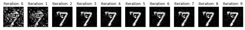
Typically, the first few iterations find counterfactuals that are out of distribution, while the later iterations make the counterfactual more sparse and interpretable.
Let’s now try to steer the counterfactual to a specific class:
[13]:
target_class = 1

cf = Counterfactual(cnn, shape=shape, target_proba=target_proba, tol=tol,
                    target_class=target_class, max_iter=max_iter, lam_init=lam_init,
                    max_lam_steps=max_lam_steps, learning_rate_init=learning_rate_init,
                    feature_range=feature_range)

explanation = start_time = time()
explanation = cf.explain(X)
print('Explanation took {:.3f} sec'.format(time() - start_time))
Explanation took 6.249 sec
Results:
[14]:
pred_class = explanation.cf['class']
proba = explanation.cf['proba'][0][pred_class]

print(f'Counterfactual prediction: {pred_class} with probability {proba}')
plt.imshow(explanation.cf['X'].reshape(28, 28));
Counterfactual prediction: 1 with probability 0.9999160766601562

As you can see, by specifying a class, the search process can’t go towards the closest class to the test instance (in this case a 9 as we saw previously), so the resulting counterfactual might be less interpretable. We can gain more insight by looking at the difference between the counterfactual and the original instance:
[15]:
plt.imshow((explanation.cf['X'] - X).reshape(28, 28));
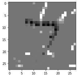
This shows that the counterfactual is stripping out the top part of the 7 to make to result in a prediction of 1 - not very surprising as the dataset has a lot of examples of diagonally slanted 1’s.
Clean up:
[16]:
os.remove('mnist_cnn.h5')