This page was generated from examples/simple_2d_drift.ipynb.

A simple drift detection example

For a simple example, we’ll use the MMD detector to check for drift on the two-dimensional binary classification problem shown previously. The MMD detector is a kernel-based method for multivariate two sample testing. Since the number of dimensions is already low, dimension reduction step is not necessary here here. For a more advanced example using the MMD detector with dimension reduction, check out the Maximum Mean Discrepancy drift detector on CIFAR-10 example.

import matplotlib.pyplot as plt
from matplotlib.colors import LinearSegmentedColormap

The true model/process is defined as:

\[\begin{split}y = \begin{cases} 1 & \text{if } x_2 > sx_1 \\ 0 & \text{otherwise} \end{cases}\end{split}\]

where the slope \(s\) is set as \(s=-1\).

import numpy as np
from scipy.stats import multivariate_normal

def true_model(X,slope=-1):
    z = slope*X[:,0]
    idx = np.argwhere(X[:,1]>z)
    y = np.zeros(X.shape[0])
    y[idx] = 1
    return y

true_slope = -1

The reference distribution is defined as a mixture of two Normal distributions:

\[P_{ref}(\mathbf{X}) = \phi_1 \mathcal{N}\left(\left[-1,-1\right]^T, \sigma^2\mathbf{I} \right) + \phi_2 \mathcal{N}\left(\left[1,1\right]^T, \sigma^2\mathbf{I} \right)\]

with the standard deviation set at \(\sigma=0.8\), and the weights set to \(\phi_1=\phi_2=0.5\). Reference data \(\mathbf{X}^{ref}\) and training data \(\mathbf{X}^{train}\) (see Note 1) can be generated by sampling from this distribution. The corresponding labels \(y^{ref}\) and \(y^{train}\) are obtained by evalulating true_model().

# Reference distribution
sigma = 0.8
phi1 = 0.5
phi2 = 0.5
ref_norm_0 = multivariate_normal([-1,-1], np.eye(2)*sigma**2)
ref_norm_1 = multivariate_normal([ 1, 1], np.eye(2)*sigma**2)

# Reference data (to initialise the detectors)
N_ref = 240
X_0 = ref_norm_0.rvs(size=int(N_ref*phi1),random_state=1)
X_1 = ref_norm_1.rvs(size=int(N_ref*phi2),random_state=1)
X_ref = np.vstack([X_0, X_1])
y_ref = true_model(X_ref,true_slope)

# Training data (to train the classifer)
N_train = 240
X_0 = ref_norm_0.rvs(size=int(N_train*phi1),random_state=0)
X_1 = ref_norm_1.rvs(size=int(N_train*phi2),random_state=0)
X_train = np.vstack([X_0, X_1])
y_train = true_model(X_train,true_slope)

To save time later on, a plotting function is defined:

plt.rcParams.update({'font.size': 16})

def plot(X,y, slope, clf=None):
    # Init plot
    fig, ax = plt.subplots(figsize=(4,4))
    #ax.axis('equal')
    ax.set_xlabel(r'$x_1$')
    ax.set_ylabel(r'$x_2$')
    ax.set_xlim([-3.5,3.5])
    ax.set_ylim([-6,3.3])

    # Plot data
    cmap = LinearSegmentedColormap.from_list('my_cmap', [(0.78,0.44,0.22), (0.22, 0.44, 0.78)], N=2)
    scat = ax.scatter(X[:,0], X[:,1],c=y,ec='k',s=70,cmap=cmap,alpha=0.7)

    # Plot true decision boundary
    xconcept = np.array(ax.get_xlim())
    ax.plot(xconcept,xconcept*slope,'k--',lw=2,alpha=0.8)

    if clf is not None:
        # Plot classifier decision boundary
        xlim = ax.get_xlim()
        ylim = ax.get_ylim()

        xx = np.linspace(xlim[0], xlim[1], 100)
        yy = np.linspace(ylim[0], ylim[1], 100)
        XX, YY = np.meshgrid(xx, yy)
        Z = clf.predict(np.c_[XX.ravel(), YY.ravel()])

        # Put the result into a color plot
        Z = Z.reshape(XX.shape)
        ax.contourf(xx, yy, Z, cmap=cmap, alpha=.3, levels=1)
        ax.contour(xx, yy, Z, colors='k', linestyles=':', linewidths=[2,0], levels=1,alpha=0.8)

    plt.show()

labels = ['No','Yes']

For a model, we choose the well-known decision tree classifier. As well as training the model, this is a good time to initialise the MMD detector with the held-out reference data \(\mathbf{X}^{ref}\) by calling:

detector = MMDDrift(X_ref, backend='pytorch', p_val=.05)

The significance threshold is set at \(\alpha=0.05\), meaning the detector will flag results as drift detected when the computed \(p\)-value is less than this i.e. \(\hat{p}< \alpha\).

# Fit decision tree classifier
from sklearn.tree import DecisionTreeClassifier
clf = DecisionTreeClassifier(max_depth=20)
clf.fit(X_train, y_train)

# Plot
plot(X_ref,y_ref,true_slope,clf=clf)

# Classifier accuracy
print('Mean training accuracy %.2f%%' %(100*clf.score(X_ref,y_ref)))

# Fit a drift detector to the training data
from alibi_detect.cd import MMDDrift
detector = MMDDrift(X_ref, backend='pytorch', p_val=.05)

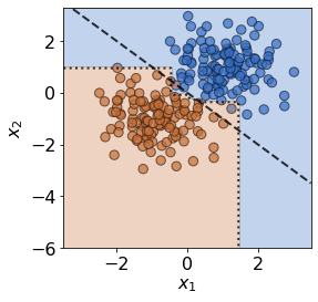
Mean training accuracy 99.17%
No GPU detected, fall back on CPU.

No drift

Before introducing drift, we first examine the case where no drift is present. We resample from the same mixture of Gaussian distributions to generate test data \(\mathbf{X}\). The individual data observations are different, but the underlying distributions are unchanged, hence no true drift is present.

N_test = 120
X_0 = ref_norm_0.rvs(size=int(N_test*phi1),random_state=2)
X_1 = ref_norm_1.rvs(size=int(N_test*phi2),random_state=2)
X_test = np.vstack([X_0, X_1])

# Plot
y_test = true_model(X_test,true_slope)
plot(X_test,y_test,true_slope,clf=clf)

# Classifier accuracy
print('Mean test accuracy %.2f%%' %(100*clf.score(X_test,y_test)))

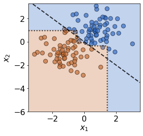
Mean test accuracy 95.00%

Unsurprisingly, the model’s mean test accuracy is relatively high. To run the detector on test data the .predict() is used:

detector.predict(X_test)

{'data': {'is_drift': 0,
  'distance': 0.0023595122654528344,
  'p_val': 0.23999999463558197,
  'threshold': 0.05,
  'distance_threshold': 0.007951605},
 'meta': {'name': 'MMDDriftTorch',
  'detector_type': 'offline',
  'data_type': None,
  'backend': 'pytorch'}}

For the test statistic \(S(\mathbf{X})\), the MMD detector uses the kernel trick to compute unbiased estimates of \(\text{MMD}^2\). The \(\text{MMD}\) is a distance-based measure between the two distributions \(P\) and \(P_{ref}\), based on the mean embeddings \(\mu\) and \(\mu_{ref}\) in a reproducing kernel Hilbert space \(F\):

\[\text{MMD}^2\left(F, P, P_{ref}\right) = \lVert \mu - \mu_{ref} \rVert^2_{F}\]

A \(p\)-value is then obtained via a permutation test on the estimates of \(\text{MMD}^2\). As expected, since we are sampling from the reference distribution \(P_{ref}(\mathbf{X})\), the detector’s prediction is 'is_drift':0 here, indicating that drift is not detected. More specifically, the detector’s \(p\)-value (p_val) is above the threshold of \(\alpha=0.05\) (threshold), indicating that no statistically significant drift has been detected. The .predict() method also returns \(\hat{S}(\mathbf{X})\) (distance_threshold), which is the threshold in terms of the test statistic \(S(\mathbf{X})\) i.e. when \(S(\mathbf{X})\ge \hat{S}(\mathbf{X})\) statistically significant drift has been detected.

Covariate and prior drift

To impose covariate drift, we apply a shift to the mean of one of the normal distributions:

\[P(\mathbf{X}) = \phi_1 \mathcal{N}\left(\left[-1\color{red}{+3},-1\color{red}{-3}\right]^T, \sigma^2\mathbf{I} \right) + \phi_2 \mathcal{N}\left(\left[1,1\right]^T, \sigma^2\mathbf{I} \right)\]

shift_norm_0 = multivariate_normal([2, -4], np.eye(2)*sigma**2)
X_0 = shift_norm_0.rvs(size=int(N_test*phi1),random_state=2)
X_1 = ref_norm_1.rvs(size=int(N_test*phi2),random_state=2)
X_test = np.vstack([X_0, X_1])

# Plot
y_test = true_model(X_test,true_slope)
plot(X_test,y_test,true_slope,clf=clf)

# Classifier accuracy
print('Mean test accuracy %.2f%%' %(100*clf.score(X_test,y_test)))

# Check for drift in covariates
pred = detector.predict(X_test)
print('Is drift? %s!' %labels[pred['data']['is_drift']])

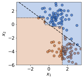
Mean test accuracy 66.67%
Is drift? Yes!

The test data has drifted into a previously unseen region of feature space, and the model is now misclassifying a number of test observations. If true test labels are available, this is easily detectable by monitoring the test accuracy. However, labels aren’t always avaiable at test time, in which case a drift detector monitoring the covariates comes in handy. In this case, the MMD detector successfully detects the covariate drift.

In a similar manner, a proxy for prior drift can be monitored by initialising a detector on labels from the reference set, and then feeding it a model’s predicted labels:

label_detector = MMDDrift(y_ref.reshape(-1,1), backend='tensorflow', p_val=.05)
y_pred = clf.predict(X_test)
label_detector.predict(y_pred.reshape(-1,1))

Concept drift

Concept drift detectors are coming soon!