This page was generated from examples/anchor_image_fashion_mnist.ipynb.

Anchor explanations for fashion MNIST

import matplotlib
%matplotlib inline
import matplotlib.pyplot as plt
import numpy as np
import tensorflow as tf
from tensorflow.keras.layers import Conv2D, Dense, Dropout, Flatten, MaxPooling2D, Input
from tensorflow.keras.models import Model
from tensorflow.keras.utils import to_categorical
from alibi.explainers import AnchorImage

Load and prepare fashion MNIST data

(x_train, y_train), (x_test, y_test) = tf.keras.datasets.fashion_mnist.load_data()
print('x_train shape:', x_train.shape, 'y_train shape:', y_train.shape)

x_train shape: (60000, 28, 28) y_train shape: (60000,)

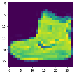
idx = 0
plt.imshow(x_train[idx]);

Scale, reshape and categorize data

x_train = x_train.astype('float32') / 255
x_test = x_test.astype('float32') / 255
x_train = np.reshape(x_train, x_train.shape + (1,))
x_test = np.reshape(x_test, x_test.shape + (1,))
print('x_train shape:', x_train.shape, 'x_test shape:', x_test.shape)
y_train = to_categorical(y_train)
y_test = to_categorical(y_test)
print('y_train shape:', y_train.shape, 'y_test shape:', y_test.shape)

x_train shape: (60000, 28, 28, 1) x_test shape: (10000, 28, 28, 1)
y_train shape: (60000, 10) y_test shape: (10000, 10)

Define CNN model

def model():
    x_in = Input(shape=(28, 28, 1))
    x = Conv2D(filters=64, kernel_size=2, padding='same', activation='relu')(x_in)
    x = MaxPooling2D(pool_size=2)(x)
    x = Dropout(0.3)(x)

    x = Conv2D(filters=32, kernel_size=2, padding='same', activation='relu')(x)
    x = MaxPooling2D(pool_size=2)(x)
    x = Dropout(0.3)(x)

    x = Flatten()(x)
    x = Dense(256, activation='relu')(x)
    x = Dropout(0.5)(x)
    x_out = Dense(10, activation='softmax')(x)

    cnn = Model(inputs=x_in, outputs=x_out)
    cnn.compile(loss='categorical_crossentropy', optimizer='adam', metrics=['accuracy'])

    return cnn

cnn = model()
cnn.summary()

Model: "model"
_________________________________________________________________
Layer (type)                 Output Shape              Param #
=================================================================
input_1 (InputLayer)         [(None, 28, 28, 1)]       0
_________________________________________________________________
conv2d (Conv2D)              (None, 28, 28, 64)        320
_________________________________________________________________
max_pooling2d (MaxPooling2D) (None, 14, 14, 64)        0
_________________________________________________________________
dropout (Dropout)            (None, 14, 14, 64)        0
_________________________________________________________________
conv2d_1 (Conv2D)            (None, 14, 14, 32)        8224
_________________________________________________________________
max_pooling2d_1 (MaxPooling2 (None, 7, 7, 32)          0
_________________________________________________________________
dropout_1 (Dropout)          (None, 7, 7, 32)          0
_________________________________________________________________
flatten (Flatten)            (None, 1568)              0
_________________________________________________________________
dense (Dense)                (None, 256)               401664
_________________________________________________________________
dropout_2 (Dropout)          (None, 256)               0
_________________________________________________________________
dense_1 (Dense)              (None, 10)                2570
=================================================================
Total params: 412,778
Trainable params: 412,778
Non-trainable params: 0
_________________________________________________________________

Train model

cnn.fit(x_train, y_train, batch_size=64, epochs=3)

Train on 60000 samples
Epoch 1/3
60000/60000 [==============================] - 29s 481us/sample - loss: 0.5932 - acc: 0.7819
Epoch 2/3
60000/60000 [==============================] - 33s 542us/sample - loss: 0.4066 - acc: 0.8506
Epoch 3/3
60000/60000 [==============================] - 32s 525us/sample - loss: 0.3624 - acc: 0.8681

<tensorflow.python.keras.callbacks.History at 0x7fae6dd5cb70>

# Evaluate the model on test set
score = cnn.evaluate(x_test, y_test, verbose=0)
print('Test accuracy: ', score[1])

Test accuracy:  0.8867

Define superpixels

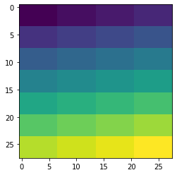
Function to generate rectangular superpixels for a given image. Alternatively, use one of the built in methods. It is important to have meaningful superpixels in order to generate a useful explanation. Please check scikit-image’s segmentation methods (felzenszwalb, slic and quickshift built in the explainer) for more information on the built in methods.

def superpixel(image, size=(4, 7)):
    segments = np.zeros([image.shape[0], image.shape[1]])
    row_idx, col_idx = np.where(segments == 0)
    for i, j in zip(row_idx, col_idx):
        segments[i, j] = int((image.shape[1]/size[1]) * (i//size[0]) + j//size[1])
    return segments

segments = superpixel(x_train[idx])
plt.imshow(segments);

Define prediction function

predict_fn = lambda x: cnn.predict(x)

Initialize anchor image explainer

image_shape = x_train[idx].shape
explainer = AnchorImage(predict_fn, image_shape, segmentation_fn=superpixel)

Explain a prediction

The explanation returns a mask with the superpixels that constitute the anchor.

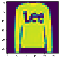
Image to be explained:

i = 1
image = x_test[i]
plt.imshow(image[:,:,0]);

Model prediction:

cnn.predict(image.reshape(1, 28, 28, 1)).argmax()

2

The predicted category correctly corresponds to the class Pullover:

Label	Description
0	T-shirt/top
1	Trouser
2	Pullover
3	Dress
4	Coat
5	Sandal
6	Shirt
7	Sneaker
8	Bag
9	Ankle boot

Generate explanation:

explanation = explainer.explain(image, threshold=.95, p_sample=.8, seed=0)

Show anchor:

plt.imshow(explanation.anchor[:,:,0]);

From the example, it looks like the end of the sleeve alone is sufficient to predict a pullover.